Chapter 2 Spatial data manipulation in R
Learning Objectives
- Join attribute data to a polygon vector file
- Select data using attribute and spatial relationships
- Reproject spatial data
- Aggregate spatial data using spatial relationships
There are a wide variety of spatial, topological, and attribute data operations we can perform with R. Lovelace et al’s recent publication1 goes into great depth about this and is highly recommended.
In this section we will look at just a few examples for libraries and functions that allow us to process spatial data in R and perform some commonly used operations.
2.1 Attribute Join
An attribute join on vector data brings tabular data into a geographic context. It refers to the process of joining data in tabular format to data in a format that holds the geometries (polygon, line, or point)2.
If you have done attribute joins of shapefiles in GIS software like ArcGIS or QGIS you know that you need a unique identifier in both the attribute table of the Shapefile and the table to be joined.
First we will load the CSV table nyc_census_tracts_pophu.csv into a tibble dataframe in R tidyverse and name it nyc_pophu for population and housing unit information.
#> spc_tbl_ [2,164 × 12] (S3: spec_tbl_df/tbl_df/tbl/data.frame)
#> $ GEOID10 : num [1:2164] 3.6e+10 3.6e+10 3.6e+10 3.6e+10 3.6e+10 ...
#> $ STATEFP : num [1:2164] 36 36 36 36 36 36 36 36 36 36 ...
#> $ COUNTYFP : chr [1:2164] "005" "005" "005" "005" ...
#> $ TRACTCE : chr [1:2164] "002300" "002701" "004100" "004800" ...
#> $ AFFGEOID : chr [1:2164] "1400000US36005002300" "1400000US36005002701" "1400000US36005004100" "1400000US36005004800" ...
#> $ POPULATION: num [1:2164] 4774 3016 6476 3999 7421 ...
#> $ MEDAGE : num [1:2164] 29 29 23 30 28 28 29 44 38 39 ...
#> $ MEDHHINC : num [1:2164] 14479 20153 18636 30301 21016 ...
#> $ MEDHOUSING: num [1:2164] 406 627 655 1066 753 ...
#> $ PCPREWAR : num [1:2164] 26.8 40.6 31.3 51.1 37.3 55.5 52 19.7 18.9 18.7 ...
#> $ MEDYRBUILT: num [1:2164] 1957 1952 1955 1942 1950 ...
#> $ DENSITY : num [1:2164] 118158 94522 90795 68668 90478 ...
#> - attr(*, "spec")=
#> .. cols(
#> .. GEOID10 = col_double(),
#> .. STATEFP = col_double(),
#> .. COUNTYFP = col_character(),
#> .. TRACTCE = col_character(),
#> .. AFFGEOID = col_character(),
#> .. POPULATION = col_double(),
#> .. MEDAGE = col_double(),
#> .. MEDHHINC = col_double(),
#> .. MEDHOUSING = col_double(),
#> .. PCPREWAR = col_double(),
#> .. MEDYRBUILT = col_double(),
#> .. DENSITY = col_double()
#> .. )
#> - attr(*, "problems")=<externalptr>2.1.1 How to do this in sf
Now let’s read the spatial data from a Shapefile into a sf object. Check out the column names of nyc_census_tracts_sf and of nyc_pophu to determine which one might contain the unique identifier for the join.
#> Reading layer `nyc_census_tracts' from data source
#> `D:\Cloud_Drive\Hunter College Dropbox\Shipeng Sun\Workspace\RSpace\R-Spatial_Book\data\nyc\nyc_census_tracts.shp'
#> using driver `ESRI Shapefile'
#> Simple feature collection with 2162 features and 10 fields
#> Geometry type: MULTIPOLYGON
#> Dimension: XY
#> Bounding box: xmin: -74.25559 ymin: 40.5021 xmax: -73.70002 ymax: 40.91526
#> Geodetic CRS: NAD83#> Classes 'sf' and 'data.frame': 2162 obs. of 11 variables:
#> $ GEOID : chr "36061000100" "36061001401" "36061000201" "36061000600" ...
#> $ STATEFP : chr "36" "36" "36" "36" ...
#> $ COUNTYFP: chr "061" "061" "061" "061" ...
#> $ TRACTCE : chr "000100" "001401" "000201" "000600" ...
#> $ AFFGEOID: chr "1400000US36061000100" "1400000US36061001401" "1400000US36061000201" "1400000US36061000600" ...
#> $ NAME : chr "1" "14.01" "2.01" "6" ...
#> $ LSAD : chr "CT" "CT" "CT" "CT" ...
#> $ ALAND : num 78638 93510 90233 240406 310039 ...
#> $ AWATER : num 0 0 75976 176018 428737 ...
#> $ CBSA : chr "New York-Newark-Jersey City, NY-NJ-PA" "New York-Newark-Jersey City, NY-NJ-PA" "New York-Newark-Jersey City, NY-NJ-PA" "New York-Newark-Jersey City, NY-NJ-PA" ...
#> $ geometry:sfc_MULTIPOLYGON of length 2162; first list element: List of 3
#> ..$ :List of 1
#> .. ..$ : num [1:25, 1:2] -74 -74 -74 -74 -74 ...
#> ..$ :List of 1
#> .. ..$ : num [1:5, 1:2] -74 -74 -74 -74 -74 ...
#> ..$ :List of 1
#> .. ..$ : num [1:14, 1:2] -74 -74 -74 -74 -74 ...
#> ..- attr(*, "class")= chr [1:3] "XY" "MULTIPOLYGON" "sfg"
#> - attr(*, "sf_column")= chr "geometry"
#> - attr(*, "agr")= Factor w/ 3 levels "constant","aggregate",..: NA NA NA NA NA NA NA NA NA NA
#> ..- attr(*, "names")= chr [1:10] "GEOID" "STATEFP" "COUNTYFP" "TRACTCE" ...To join the nyc_pophu data frame with nyc_census_tracts_sf we can use merge in the base package like this:
nyc_sf_merged <- base::merge(nyc_census_tracts_sf, nyc_pophu, by.x = "GEOID", by.y = "GEOID10")
names(nyc_sf_merged) #> [1] "GEOID" "STATEFP.x" "COUNTYFP.x" "TRACTCE.x" "AFFGEOID.x"
#> [6] "NAME" "LSAD" "ALAND" "AWATER" "CBSA"
#> [11] "STATEFP.y" "COUNTYFP.y" "TRACTCE.y" "AFFGEOID.y" "POPULATION"
#> [16] "MEDAGE" "MEDHHINC" "MEDHOUSING" "PCPREWAR" "MEDYRBUILT"
#> [21] "DENSITY" "geometry"We see the new attribute columns added, as well as the geometry column.
# A basic plot to verify the data: use zcol to choose a subset of the data to plot
mapview(nyc_sf_merged, zcol=c('POPULATION','MEDHHINC'))Alternatively, we can use tidyverse function join (left_join, right_join, inner_join etc) to conduct the task. Note that this requires the two matching columns being the same type.
2.2 Attribute Selection (or non-spatial subsetting)
sf objects are also tidyverse compatible data.frame. Using dplyr::filter, we can easy select a subset (rows) from sf data using tidyverse functions like dplyr::filter with logical expressions. The dplyr::select can select columns.
high_income_tracts <- nyc_sf_merged %>% dplyr::filter(MEDHHINC > 80000)
plot(nyc_sf_merged %>% st_geometry(), col='NA', border='lightblue', lwd=0.2)
high_income_tracts %>% st_geometry() %>% plot(col='grey', border='NA', add=TRUE)
2.3 Spatial Query
To perform spatial query, we must first understand spatial relationships in spatial analysis and GIScience. An excellent source for these relationships is GITTA Spatial Queries
The most useful spatial (or topological) relationships are illustrated below.
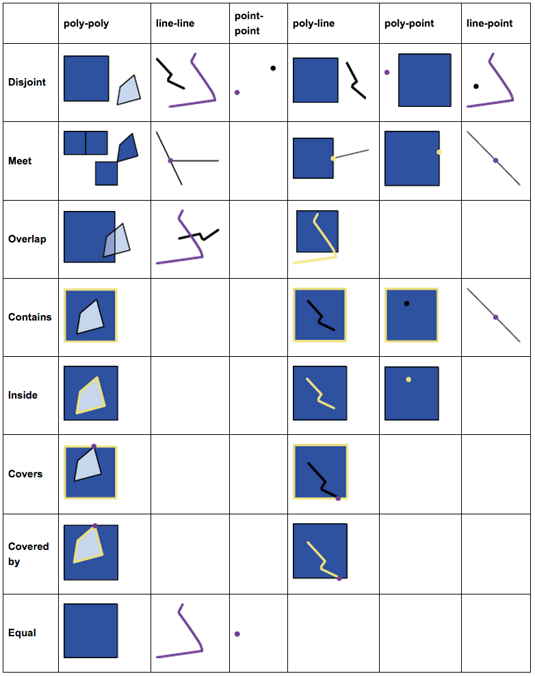
FIGURE 2.1: Spatial Relations
And these basic relations form a hierarchy. For example, the intersects relationship actually has a few subtypes like meet (or touch), overlap, and contain, etc. Anything that is not disjoint would be an intersects.
FIGURE 2.2: Hierarchy of Spatial Relations
Naming rules for spatial functions
- sf, as well as ST_SQL in PostGIS, uses verbs for functions of spatial relationships and use nouns for functions of spatial operations.
- Spatial relationship functions like st_overlaps, st_covers, and st_intersects examine the topological relationships between spatial objects.
- Of course, some functions named by prepositions and adjectives like st_within and st_equal are only meaningful for spatial relationships.
- Spatial relationship functions do not produce new geometries. They just tell use their relationships, with which we can conduct query, selection, and aggregation.
- By contrast, spatial operations will create new geometries. For example, st_intersection will produce new geometries in sf classes.
For the next example our goal is to select all census tracts that are adjacent to the central park.
Think about this for a moment – what might be the steps you’d follow?
## How about:
# 1. Get the census tract polygons.
# 2. Find the census tract that contains the central park.
# 3. Select all census tract polygons that intersect with or touch the central park tract2.3.1 Using the sf package
We will use nyc_sf_merged for the census tract polygons. Using a desktop GIS or mapview package in R, we can easily find out the GEOID of the central park tract is 36061014300.
First, let’s use non-spatial query to find the central park census tract.
# Note the GEOID column is a numeric type.
central_partk <- nyc_sf_merged %>% filter(GEOID == 36061014300)Now we can use this central_park to select all census tract polygons that intersect with the tract. In order to determine the polygons we use st_intersects, a geometric binary which returns a vector of logical values, which we we can use for subsetting. Note the difference to st_intersection, which performs a geometric operation and creates a new sf object which cuts out the area of the buffer from the polygons a like cookie cutter.
Let us try this:
central_park_intersects <- st_intersects(central_partk, nyc_sf_merged)
class(central_park_intersects)We have created a sgbp object, which is a “Sparse Geometry Binary Predicate”. It is a so called sparse matrix, which is a list with integer vectors only holding the indices for each polygon that intersects. In our case we only have one vector, because we only intersect with one buffer polygon, so we can extract this first vector with central_park_intersects[[1]] and use it for subsetting:
# Subsetting using the results
nyc_sel_sf <- nyc_sf_merged[central_park_intersects[[1]],]
# or in tidyverse style
nyc_sel_sf <- nyc_sf_merged %>% dplyr::slice(central_park_intersects[[1]])
# plot
plot(st_geometry(nyc_sf_merged), border="#aaaaaa", main="Census tracts near Central Park")
plot(st_geometry(nyc_sel_sf), add=T, col="lightpink")
plot(st_geometry(nyc_sel_sf), add=T, col=NA, border= 'lightgrey',lwd = 1)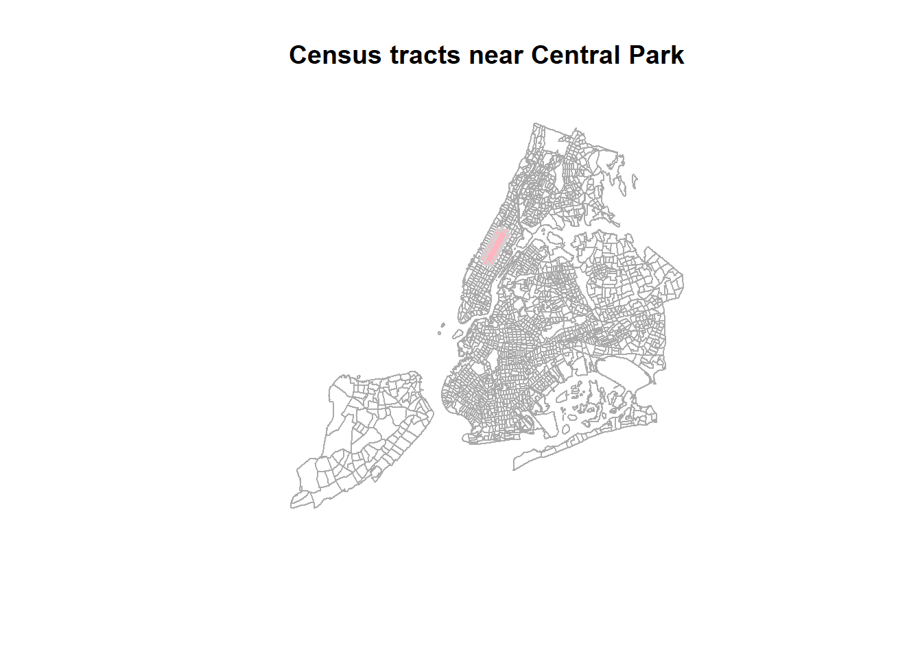
2.4 Reprojecting or Projection Transform
Occasionally we may have to change the coordinates of our spatial object into a new Coordinate Reference System (CRS).
2.4.1 Transform or reproject sf objects
Let us check nyc_sf_merged object and reproject it to a local projection in State Plane Long Island, that is the local map projection the NYC.
#> Coordinate Reference System:
#> User input: NAD83
#> wkt:
#> GEOGCRS["NAD83",
#> DATUM["North American Datum 1983",
#> ELLIPSOID["GRS 1980",6378137,298.257222101,
#> LENGTHUNIT["metre",1]]],
#> PRIMEM["Greenwich",0,
#> ANGLEUNIT["degree",0.0174532925199433]],
#> CS[ellipsoidal,2],
#> AXIS["latitude",north,
#> ORDER[1],
#> ANGLEUNIT["degree",0.0174532925199433]],
#> AXIS["longitude",east,
#> ORDER[2],
#> ANGLEUNIT["degree",0.0174532925199433]],
#> ID["EPSG",4269]]# then we transform/reproject it to SPCS Long Island, 2831
nyc_sf_2831 <- st_transform(nyc_sf_merged, 2831)
st_crs(nyc_sf_2831)#> Coordinate Reference System:
#> User input: EPSG:2831
#> wkt:
#> PROJCRS["NAD83(HARN) / New York Long Island",
#> BASEGEOGCRS["NAD83(HARN)",
#> DATUM["NAD83 (High Accuracy Reference Network)",
#> ELLIPSOID["GRS 1980",6378137,298.257222101,
#> LENGTHUNIT["metre",1]]],
#> PRIMEM["Greenwich",0,
#> ANGLEUNIT["degree",0.0174532925199433]],
#> ID["EPSG",4152]],
#> CONVERSION["SPCS83 New York Long Island zone (meter)",
#> METHOD["Lambert Conic Conformal (2SP)",
#> ID["EPSG",9802]],
#> PARAMETER["Latitude of false origin",40.1666666666667,
#> ANGLEUNIT["degree",0.0174532925199433],
#> ID["EPSG",8821]],
#> PARAMETER["Longitude of false origin",-74,
#> ANGLEUNIT["degree",0.0174532925199433],
#> ID["EPSG",8822]],
#> PARAMETER["Latitude of 1st standard parallel",41.0333333333333,
#> ANGLEUNIT["degree",0.0174532925199433],
#> ID["EPSG",8823]],
#> PARAMETER["Latitude of 2nd standard parallel",40.6666666666667,
#> ANGLEUNIT["degree",0.0174532925199433],
#> ID["EPSG",8824]],
#> PARAMETER["Easting at false origin",300000,
#> LENGTHUNIT["metre",1],
#> ID["EPSG",8826]],
#> PARAMETER["Northing at false origin",0,
#> LENGTHUNIT["metre",1],
#> ID["EPSG",8827]]],
#> CS[Cartesian,2],
#> AXIS["easting (X)",east,
#> ORDER[1],
#> LENGTHUNIT["metre",1]],
#> AXIS["northing (Y)",north,
#> ORDER[2],
#> LENGTHUNIT["metre",1]],
#> USAGE[
#> SCOPE["Engineering survey, topographic mapping."],
#> AREA["United States (USA) - New York - counties of Bronx; Kings; Nassau; New York; Queens; Richmond; Suffolk."],
#> BBOX[40.47,-74.26,41.3,-71.8]],
#> ID["EPSG",2831]]We see that the CRS are different for the two. One is geographic coordinate systems (longitude, latitude) using NAD83 and the other is New York State Plane Long Island.
We can also see the proj4 strings of the two.
: we have +proj=lcc... and +proj=longlat.... LCC refers to Lambert Conic Conformal, which is a projected coordinate system with numeric units.
We can use the st_bbox() method from the sf package to compare the coordinates before and after transformation and confirm that we actually have transformed them. st_bbox() returns the min and max values of the two dimensions of a sf spatial object.
#> xmin ymin xmax ymax
#> -74.25559 40.50210 -73.70002 40.91526#> xmin ymin xmax ymax
#> 278336.44 37278.33 325338.38 83132.41We can also compare them visually with:
par(mfrow=c(1,2))
plot(st_geometry(nyc_sf_merged), axes=TRUE, main = "before transform - latlon")
plot(st_geometry(nyc_sf_2831), axes=TRUE, main = "after transform - lcc")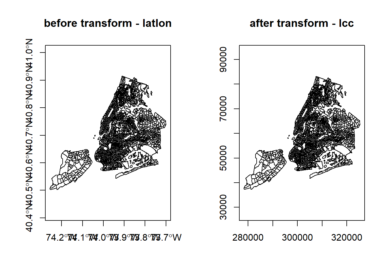
Lastly, let us save the reprojected file as nyc_tracts_2831 Shapefile, as we may use it later on.
Set CRS and Reproject (transform)
- Assigning a new CRS to a spatial object does not change its coordinates but the CRS determines how the software understand the coordinates. So, we must choose and set a CRS that is consistent with the coordinates. Otherwise, the coordinates will be misinterpreted.
- Reprojecting spatial data with st_transform and gTransform really changes the underlying coordinates, which we can see from the bbox values.
- In either case, the CRS must be consistent with the coordinates. It is a good practice to check projected spatial data against a basemap or a correctly referenced map to verify its CRS.
- SpatialReference.org is a very good source for CRS information.
- Some commonly used reference systems
- US 48 Contiguous States: Albers Equal Area (ESRI:102003), Lambert Conformal (ESRI:102004)
- New York State: UTM 18N (EPSG 3725, 3748, 26918)
- New York City: State Plane Long Island (EPSG 2263, 2831, 3627)
2.4.2 Spatial Query with Reprojection
Another scenario where we need to transform spatial data into a different projection is to apply distances. This is because local projections tend to minimize distortion and they also use units like meter or feet. Here we use a distance buffer example to illustrate both transformation/reprojection and spatial query. In this example, we try to find the noise complaint within 200 meter from Hunter College, 09/01/2019 to 09/01/2020.
First, we search the geographic coordinates of Hunter College and find (-73.9645, 40.7678). Then, we create a spatial object for this location. As we don’t really use any attribute information for this location, a sfc object is sufficient.
# make a simple feature point with CRS
hunter_college_sfc <- st_sfc(st_point(c(-73.9645, 40.7678)), crs = 4269)
# Verify the location using mapview with basemap or ggmaps
mapview(hunter_college_sfc)We can also use what we learned earlier to directly create a sf object.
# make a simple feature point with CRS
hunter_college_sf <- st_as_sf(data.frame(x=-73.9645, y=40.7678), coords = c('x','y'), crs = 4269)
# Verify the location using mapview with basemap or ggmaps
mapview(hunter_college_sf)Now, let’s read the Manhattan noise data and check on their coordinate systems. If they have the same CRS with a unit of meter, we can use them directly. Otherwise, we have to convert them to a local map projection with a meter unit.
man_noise_sf <- sf::st_read('data/nyc/ManhattanNoise.shp')
st_crs(hunter_college_sf)
st_crs(man_noise_sf)It turns out both use geographic coordinates with a unit of decimal degree. But one is using WGS84 (4326) and the other is using NAD83 (4269). Although they are very similar to each other, none of them have a unit of meter. So, we must convert both to the same CRS using New York Long Island (State Plain Coordinate System, SPCS) with a unit of meter. The SRID is 2831. Note 2263 is also New York Long Island, but its unit is feet.
To avoid saving all the intermediate results, we use pipe %>% to get the buffer and to conduct the spatial query.
hunter_college_sf %>% sf::st_transform(2831) %>% # transform the data to 2831
sf::st_buffer(200) %>% # create the buffer
sf::st_intersects(man_noise_sf # intersects with the transformed noise data
%>% st_transform(2831)) %>%
magrittr::extract2(., 1) %>% # Get the indices of the noise points within 200 meter buffer
dplyr::slice(man_noise_sf, .) %>% # Get those noise points
mapview::mapview() # Map them out using a simple interactive mapThis chunk of code may be difficult to understand. You can break it down and explicitly save the intermediate data using variables.
2.5 Spatial Join and Aggregation: Points in Polygons
Now that we have both noise and census tracts we will forge ahead and ask for the density of noise complaint for each census tract in Manhattan: \(\frac{{noise complaints}}{area}\)
To achieve this this we join the points of noise complaints to the census tract polygon and count them up for each polygon. You might be familiar with this operation from ArcGIS, QGIS, or other GIS packages. Note that for topological relationships not based on distances, it will work as long as both data have the same coordinate systems.
Essentially, spatial join is to relate or match geographic features by their spatial relationships. For example, we want to get the total number of bus stops (points) in each neighborhood (polygons). Then we can use spatial join to find out all the points within each neighborhood. Then we can summarize all these points such as their quantity to the neighborhood. This can be achieved by using sf::st_join(sfNeighborhood, sfBusstops, join=st_contains, left=TRUE). In the results, we will see combinations of each neighborhood and every bus stop the neighborhood contains.
2.5.1 With sf
We will use piping to build up our object in the following way. First we calculate the area for each tract. We use the st_area function on the geometry column and add the result.
nyc_census_tracts_sf %>%
filter(COUNTYFP == '061') %>%
mutate(tract_area = st_area(geometry)) %>%
head()Next, we use st_join to perform a spatial join with the points:
nyc_census_tracts_sf %>%
filter(COUNTYFP == '061') %>%
mutate(tract_area = st_area(geometry)) %>%
st_transform(4326) %>%
st_join(man_noise_sf) %>%
head()By default, st_join uses st_intersects for the join parameter. But we can also use more specific join types like st_within or st_contains and whether to use it as a left join. Check out the documentation of st_join for more details. On the R console, you can type ?sf::st_join to open the documentation.
Note: some join types are not symmetric such as st_contains. As a result, st_join(sfA, sfB, join= st_contains) will be very different from st_join(sfB, sfA, join = st_contains). For the first one, the match will be whether features in sfA contain features in sfB. By default, st_join is a left join, meaning all records of the fist parameter will always be kept. When the left parameter is set to FALSE, it will become an inner join.
Now we can group by a variable that uniquely identifies the census tracts, (we choose GEOID) and use summarize to count the points for each tract and calculate the rate of noise complaints. Since the area unit of the census tract is sq meter, we can multiply the areas by 1,000,000 to get sq km. We also need to carry over the area, which we can use max, min, mean, or unique as all the values are the same for the same census tract.
We also assign the output to a new object noise_rate.
noise_rate_sf <- nyc_census_tracts_sf %>%
filter(COUNTYFP == '061') %>%
mutate(tract_area = st_area(geometry)) %>%
st_transform(4326) %>%
st_join(man_noise_sf) %>%
group_by(GEOID) %>%
summarize(n_noise = n(),
tract_area = max(tract_area),
noise_rate = n_noise/tract_area * 1e6) And here is a simple plot:
Finally, we write this out for later:
2.5.2 sp - sf comparison
| how to.. | for sp objects | for sf objects |
|---|---|---|
| join attributes | sp::merge() |
dplyr::*_join() (also sf::merge()) |
| reproject | spTransform() |
st_transform() |
| retrieve (or assign) CRS | proj4string() |
st_crs() |
| count points in polygons | aggregate() or over() |
st_within() or aggregate() |
| buffer | rgeos::gBuffer() (separate package) |
st_buffer() |
| select by location | g* functions from rgeos |
st_* geos functions in sf |
Here are some additional packages that use vector data:
2.6 Spatial Operations
2.6.1 Spatial Measures
This type of operations measure certain values from spatial objects. For example, we can derive the boundary box and centroid using sf::st_bbox and sf::st_centroid. More basic measures are areas and length with sf::st_area and sf::st_length.
2.6.2 Geometric Operations
More interestingly, we can conduct certain geometric operations such as buffer and overlay. In spatial analysis, overlay contains a few types.
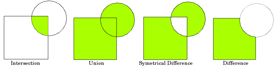
FIGURE 2.3: Overlay Types
And this web page has an excellent explanation to the spatial operations on vector data, including buffer, operations involving one (unary) or multiple layers of spatial objects.
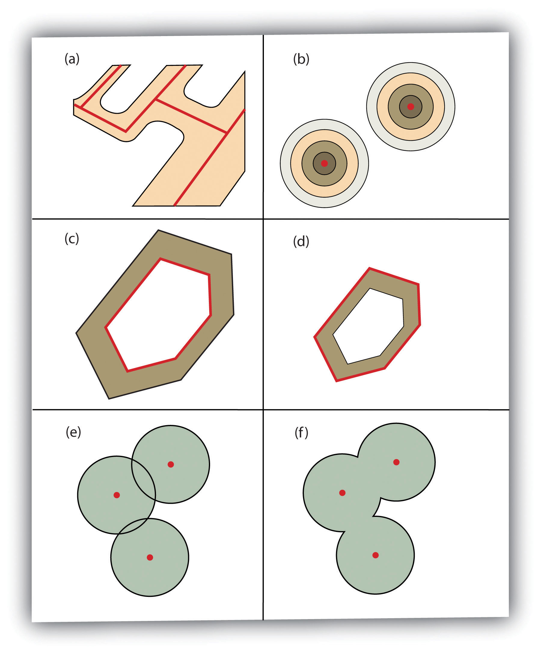
FIGURE 2.4: Buffer Options: (a) Variable Width Buffers, (b) Multiple Ring Buffers, (c) Doughnut Buffer, (d) Setback Buffer, (e) Nondissolved Buffer, (f) Dissolved Buffer
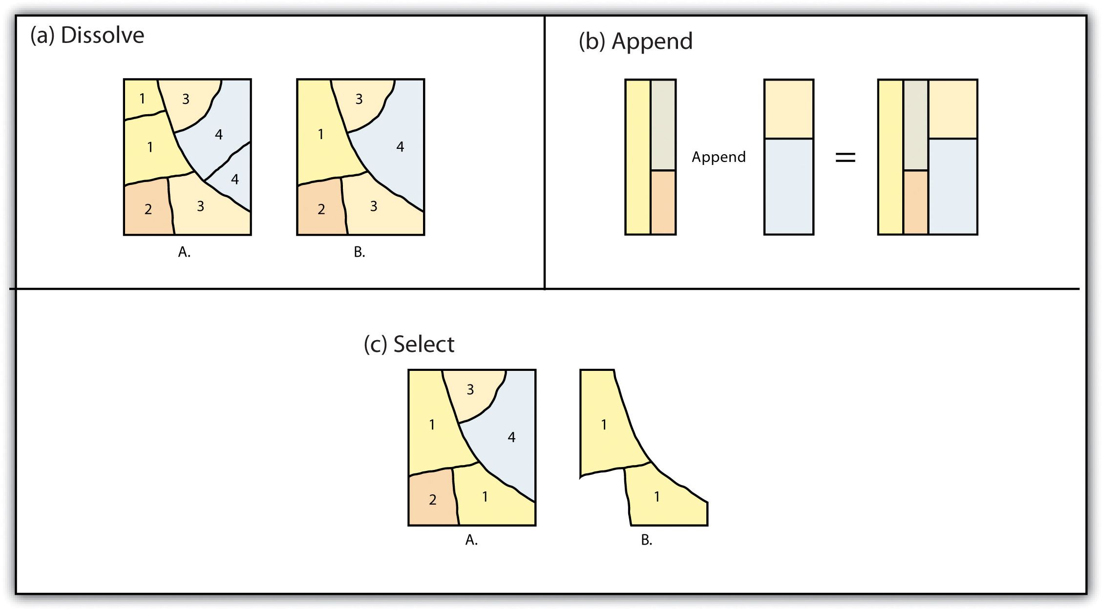
FIGURE 2.5: Single Layer Geometric Operations
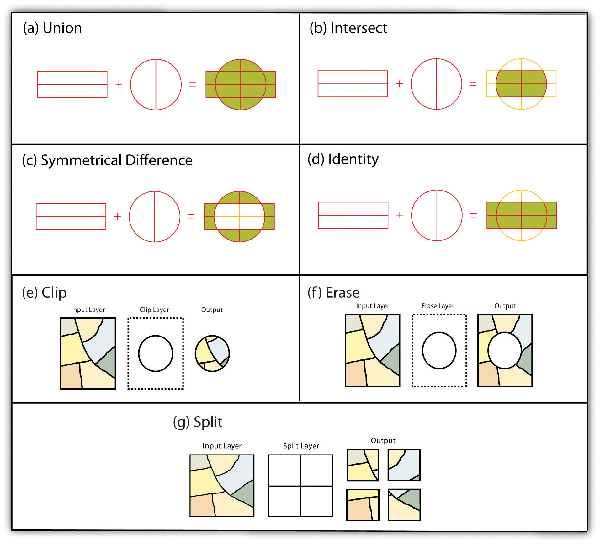
FIGURE 2.6: Multiple Layer Geometric Operations
Self Exercise
- Think about how to conduct these spatial operations using basic sf st_ and tidyverse functions.
- Dissolve: merge (data.frame), dplyr::group_by, st_union
- Append: dplyr::bind_rows, st_combine (may not give you what you expect, though)
- Identity: st_union and then st_intersection
- Erase: st_difference
- Split: st_intersection by feature ID
Geometric operations are algorithmically difficult and computationally expensive. So, quite often, results are not what we expected. More mature packages perform better. In this case, sp-family packages are better than sf-family.
buf_sf <- hunter_college_sf %>% sf::st_transform(2831) %>% # reproject the data to 2831
sf::st_buffer(800) # create the buffer
man_tracts_sf <- nyc_census_tracts_sf %>%
st_transform(2831) %>%
filter(COUNTYFP == '061')
buf_sel_sf <- buf_sf %>%
sf::st_intersects(man_tracts_sf) %>% # intersects with the transformed noise data
magrittr::extract2(., 1) %>% # Get the indices of the noise points within 200 meter buffer
dplyr::slice(man_tracts_sf, .)
par(mfrow=c(1,2), mar = c(4, 0.1, 0.8, 0.1))
plot(buf_sf %>% st_geometry(),
col='grey',
main = 'Buffer Geometry')
plot(buf_sel_sf %>% st_geometry(),
col='lightskyblue2',
main="Polygons")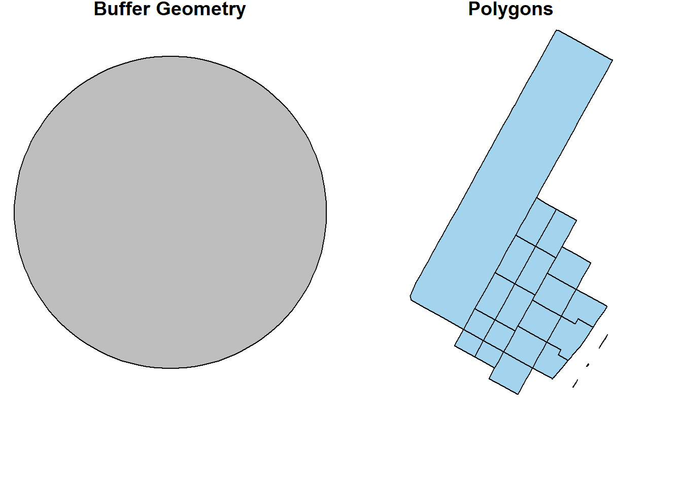
st_union(buf_sel_sf, buf_sf,by_feature = TRUE) %>%
st_geometry() %>%
plot(col='lightskyblue1', main = 'sf::st_union by feature')
rgeos::gUnion(buf_sf %>% sf::as_Spatial(),
buf_sel_sf %>% sf::as_Spatial(),
byid = TRUE) %>%
plot(col='lightpink', main = 'rgeos::gUnion (sp) by feature')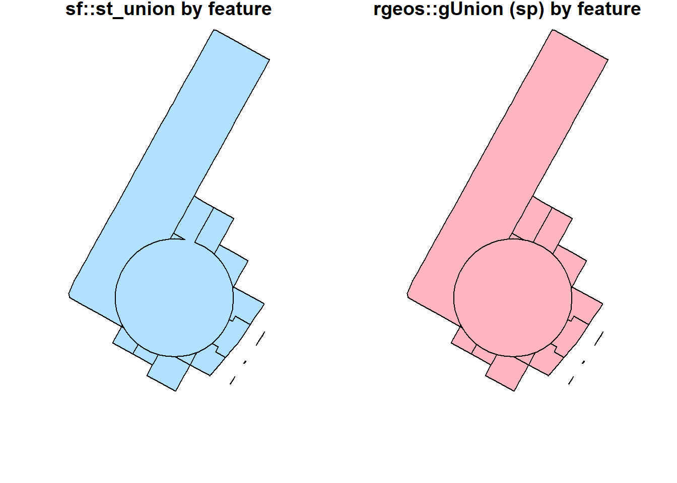
st_union(buf_sel_sf, buf_sf,by_feature = FALSE) %>%
st_geometry() %>%
plot(col='lightskyblue1', main = 'sf::st_union')
rgeos::gUnion(buf_sf %>% sf::as_Spatial(),
buf_sel_sf %>% sf::as_Spatial()) %>%
plot(col='lightpink', main = 'rgeos::gUnion (sp)')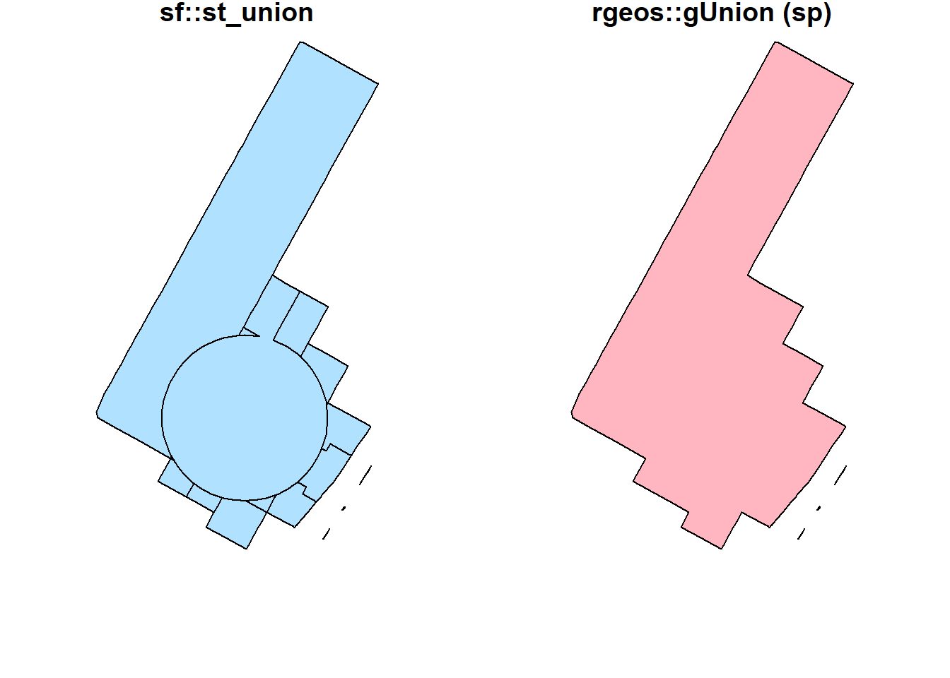
st_intersection(buf_sel_sf, buf_sf) %>%
st_geometry() %>%
plot(col='lightskyblue1', main = 'sf::st_intersection')
st_difference(buf_sel_sf, buf_sf) %>% st_geometry() %>%
plot(col='lightskyblue1',main = 'sf::st_difference')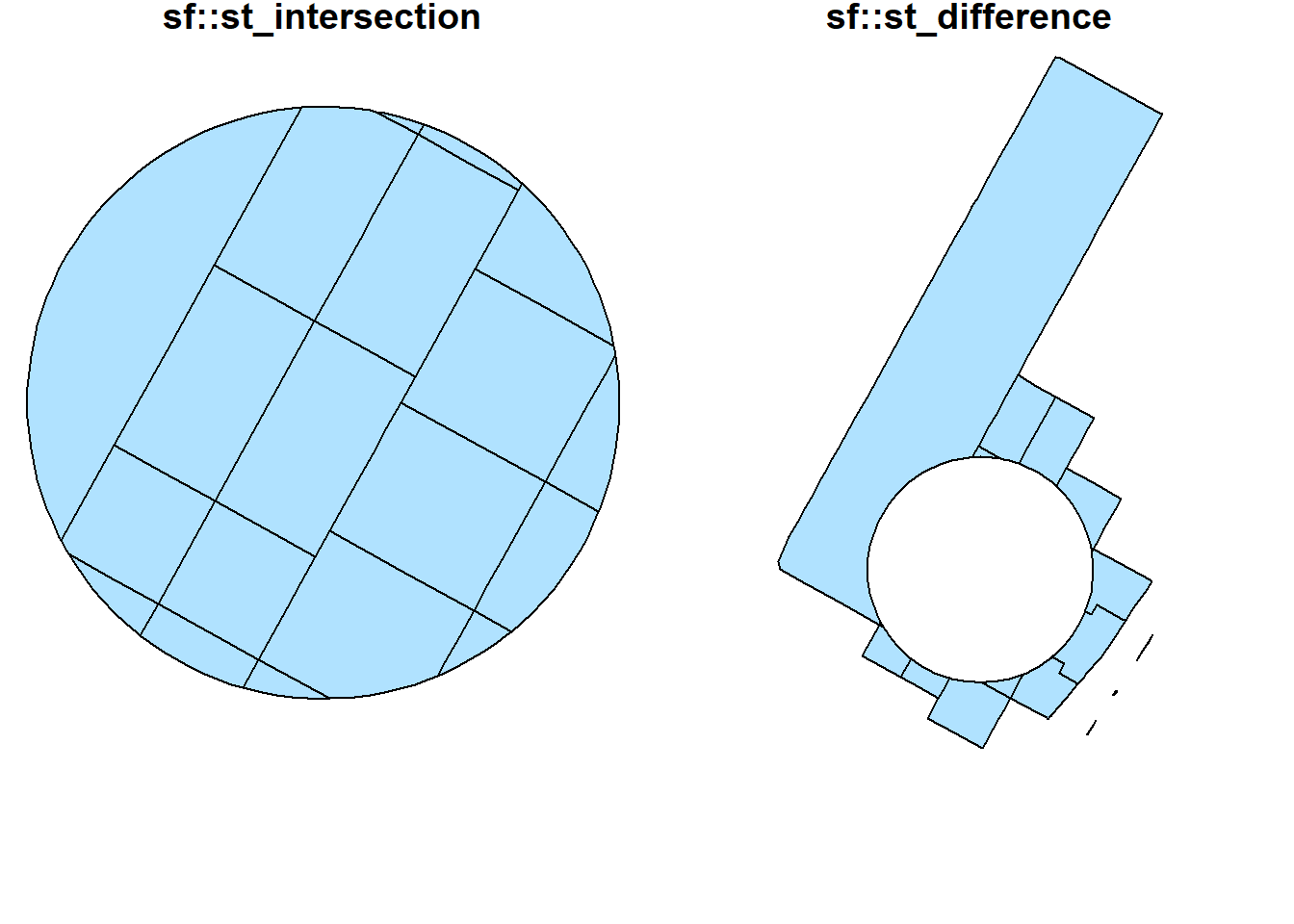
st_sym_difference(buf_sel_sf, buf_sf) %>%
st_geometry() %>%
plot(col='lightskyblue1',main = 'sf::st_sym_difference')
rgeos::gSymdifference(buf_sf %>% sf::as_Spatial(),
buf_sel_sf %>% sf::as_Spatial(),
drop_lower_td = TRUE) %>%
plot(col='lightpink', main = 'rgeos::gSymdifference (sp)')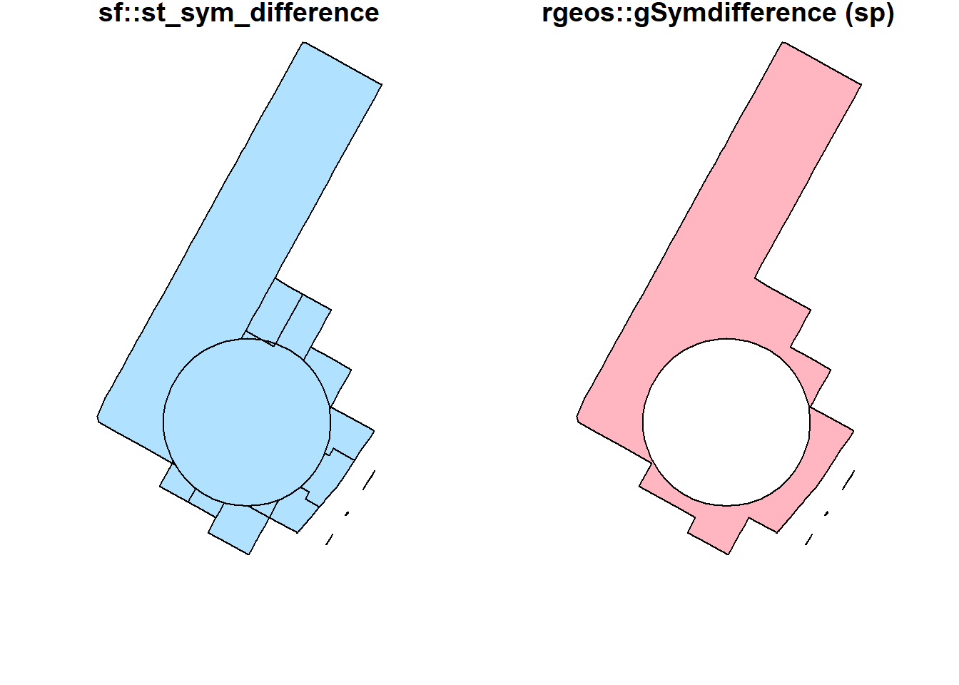
Interestingly, the raster package seems to have better intersect and union methods. Results from these methods are similar to what popular GIS software like ArcGIS produces. More importantly, they keep all the attributes from both layers.
par(mfrow=c(1,2), mar = c(4, 0.1, 0.8, 0.1));
raster::union(buf_sf %>% sf::st_geometry() %>% sf::as_Spatial(),
buf_sel_sf %>% sf::st_geometry() %>% sf::as_Spatial()) %>%
plot(col='lightpink', main = 'raster::union');
raster::intersect(buf_sf %>% sf::st_geometry() %>% sf::as_Spatial(),
buf_sel_sf %>% sf::st_geometry() %>% sf::as_Spatial()) %>%
plot(col='lightpink', main = 'raster::intersect')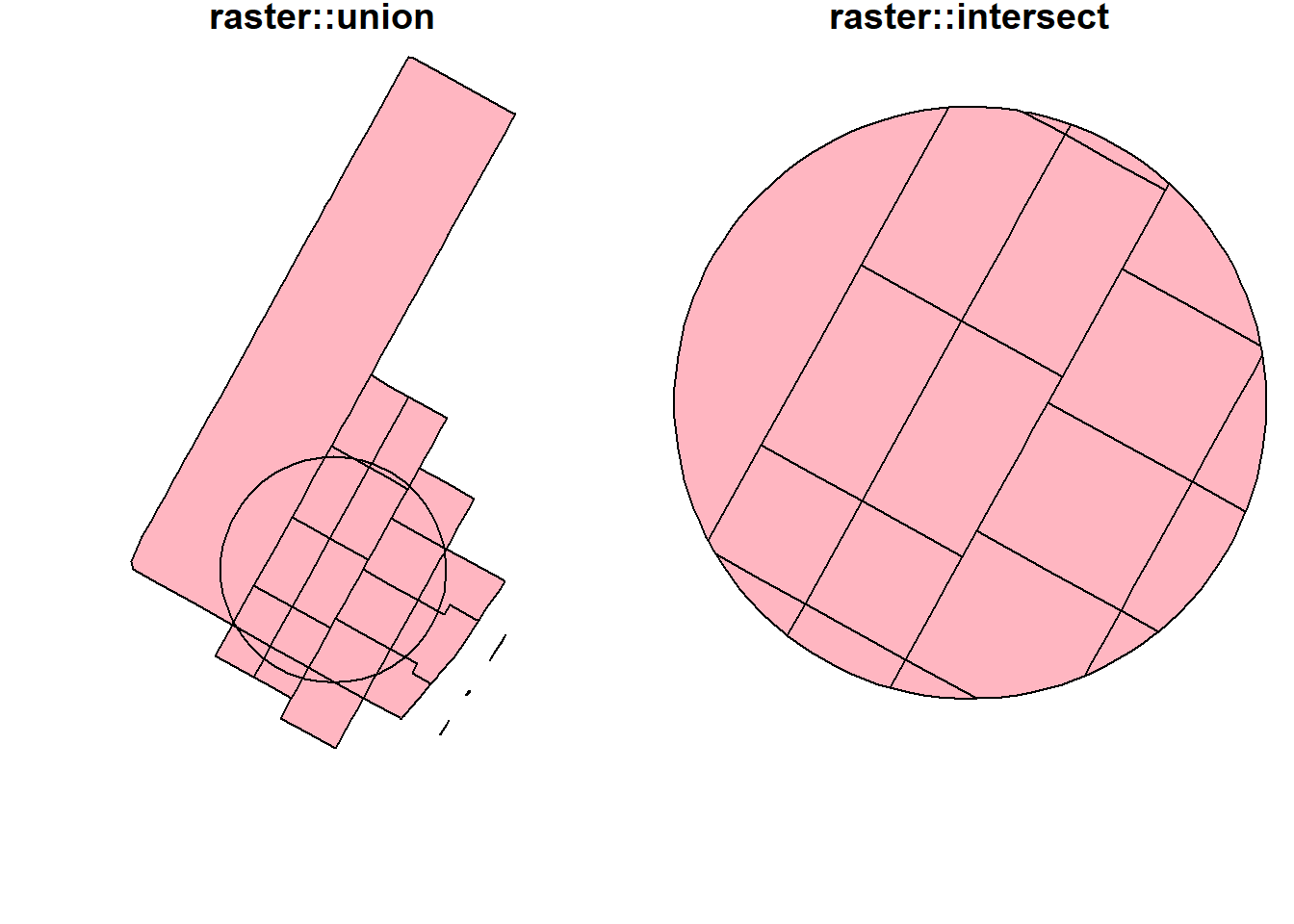
To visualize all these different operations with the original dataset.
# Various types of spatial operations
par(mfrow=c(1,2), mar = c(4, 0.1, 0.8, 0.1))
plot(st_geometry(man_tracts_sf), border="#aaaaaa", main="Buffer Geometry")
plot(buf_sf %>% st_geometry(),
col='grey',
add=T)
plot(st_geometry(man_tracts_sf), border="#aaaaaa", main="Polygons")
plot(buf_sel_sf %>% st_geometry(),
col='lightskyblue2',
add=T)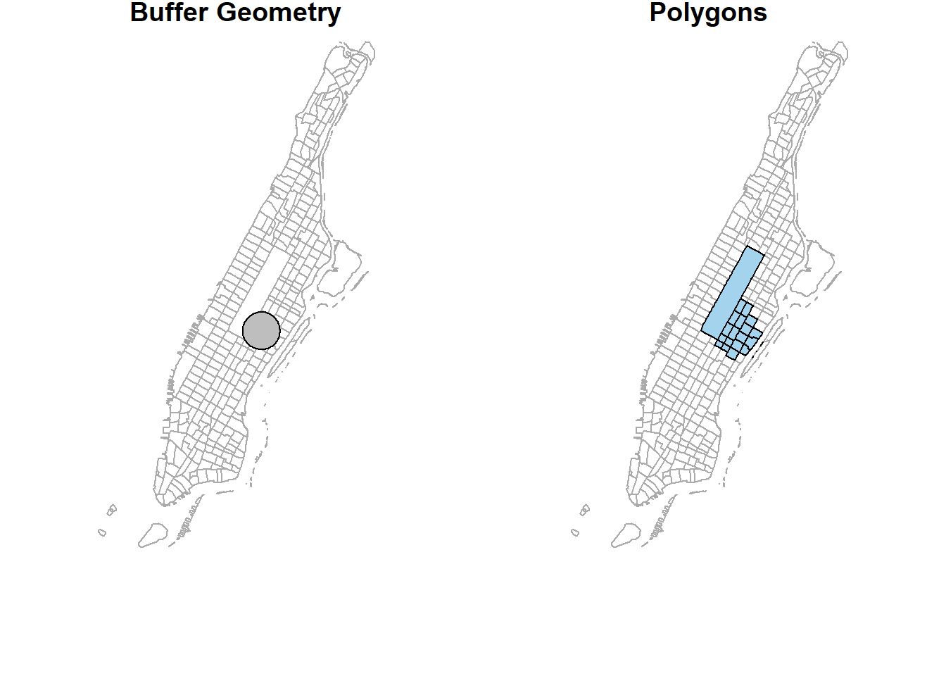
plot(st_geometry(man_tracts_sf), border="#aaaaaa", main="sf::st_union by feature")
st_union(buf_sel_sf, buf_sf,by_feature = TRUE) %>%
st_geometry() %>%
plot(col='lightskyblue1', add = T)
plot(st_geometry(man_tracts_sf), border="#aaaaaa", main='rgeos::gUnion (sp) by feature')
rgeos::gUnion(buf_sf %>% sf::as_Spatial(),
buf_sel_sf %>% sf::as_Spatial(),
byid = TRUE) %>%
plot(col='lightpink', add = T)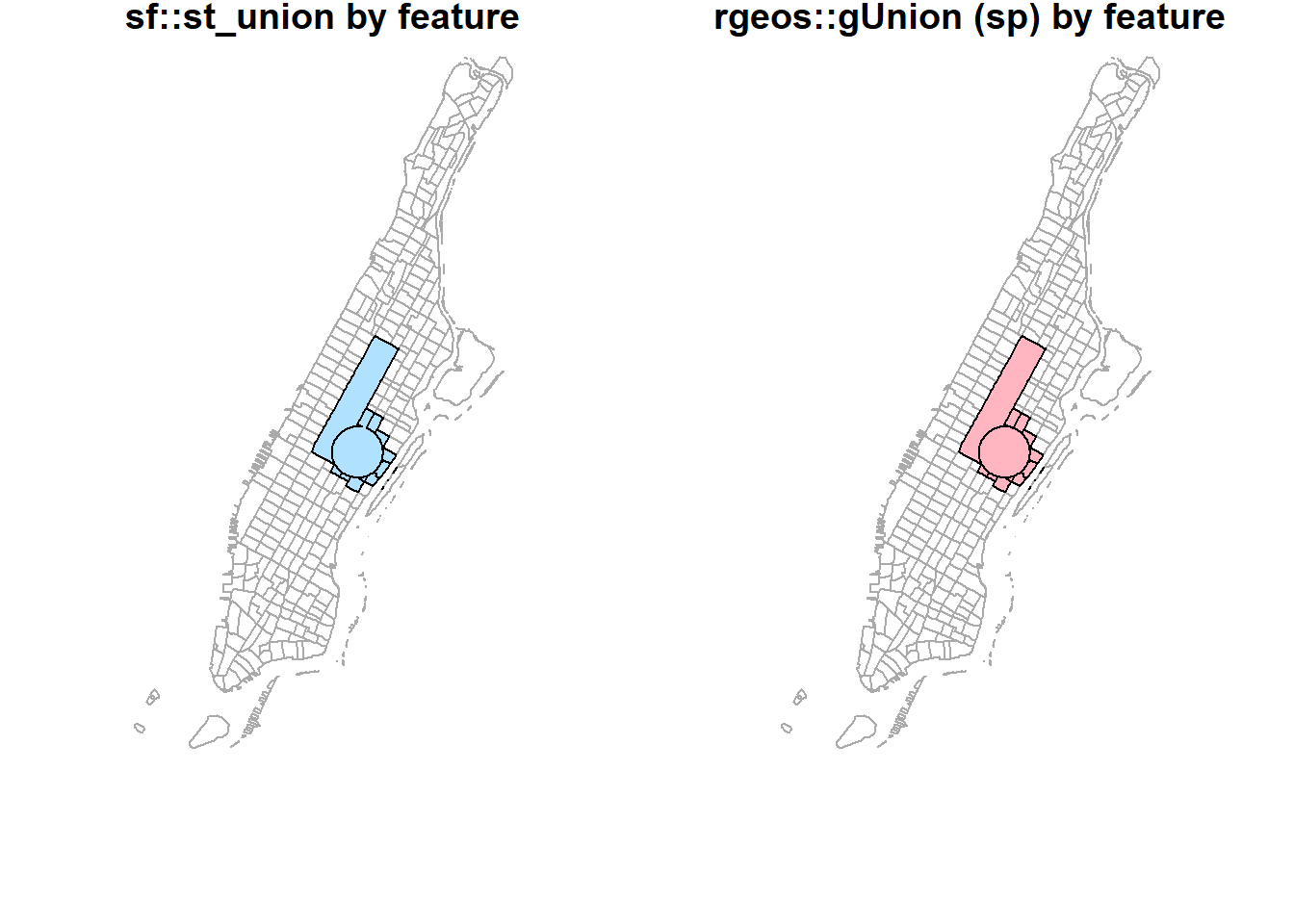
plot(st_geometry(man_tracts_sf), border="#aaaaaa", main='sf::st_untion')
st_union(buf_sel_sf, buf_sf,by_feature = FALSE) %>%
st_geometry() %>%
plot(col='lightskyblue1', add = T)
plot(st_geometry(man_tracts_sf), border="#aaaaaa", main='rgeos::gUnion (sp)')
rgeos::gUnion(buf_sf %>% sf::as_Spatial(),
buf_sel_sf %>% sf::as_Spatial()) %>%
plot(col='lightpink', add = T)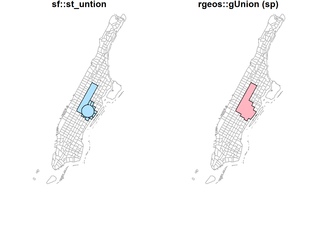
plot(st_geometry(man_tracts_sf), border="#aaaaaa", main='sf::st_intersection')
st_intersection(buf_sel_sf, buf_sf) %>%
st_geometry() %>%
plot(col='lightskyblue1', add = T)
plot(st_geometry(man_tracts_sf), border="#aaaaaa", main='sf::st_difference')
st_difference(buf_sel_sf, buf_sf) %>% st_geometry() %>%
plot(col='lightskyblue1', add = T)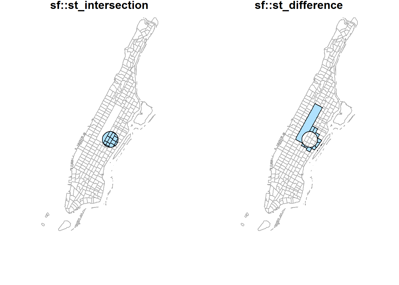
plot(st_geometry(man_tracts_sf), border="#aaaaaa", main='sf::st_sym_difference')
st_sym_difference(buf_sel_sf, buf_sf) %>%
st_geometry() %>%
plot(col='lightskyblue1', add = T)
plot(st_geometry(man_tracts_sf), border="#aaaaaa", main='rgeos::gSysdifference (sp)')
rgeos::gSymdifference(buf_sf %>% sf::as_Spatial(),
buf_sel_sf %>% sf::as_Spatial(),
drop_lower_td = TRUE) %>%
plot(col='lightpink', add = T)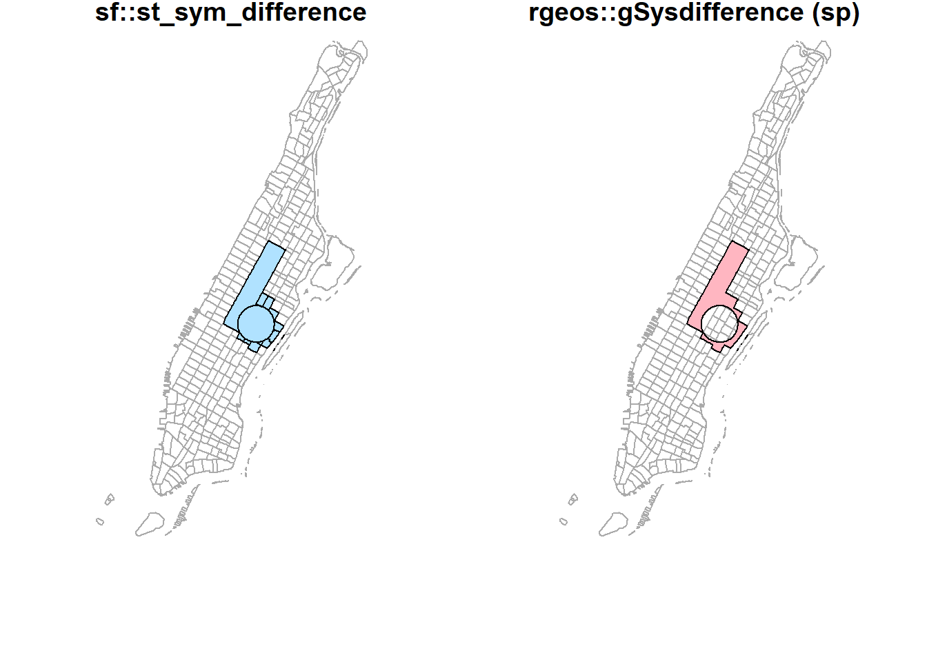
par(mfrow=c(1,2), mar = c(4, 0.1, 0.8, 0.1))
plot(st_geometry(man_tracts_sf), border="#aaaaaa", main='raster::union')
raster::union(buf_sf %>% sf::st_geometry() %>% sf::as_Spatial(),
buf_sel_sf %>% sf::st_geometry() %>% sf::as_Spatial()) %>%
plot(col='lightpink', add = T)
plot(st_geometry(man_tracts_sf), border="#aaaaaa", main='raster::instersect')
raster::intersect(buf_sf %>% sf::st_geometry() %>% sf::as_Spatial(),
buf_sel_sf %>% sf::st_geometry() %>% sf::as_Spatial()) %>%
plot(col='lightpink', add = T)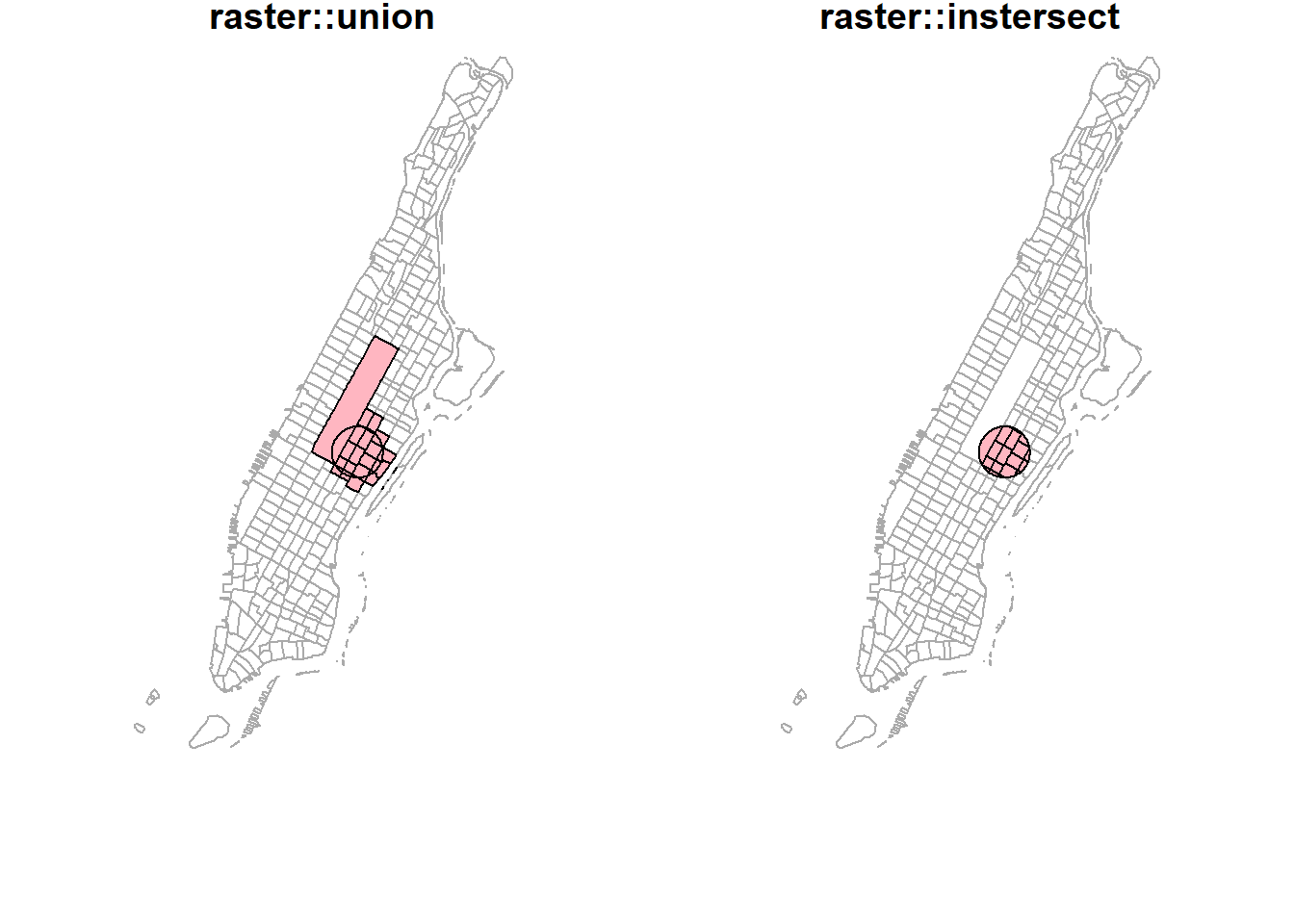
Earlier, we used group_by + summarize (sf) and aggregate (sp) to conduct spatial aggregation or spatial join. When these functions apply to a single spatial object (unary operations), they could do the dissolve. Note that those internal “sliver” polygons are caused by inaccurate boundaries. For example, two neighboring polygons should have exactly the same boundary at where they touch. But if not, those sliver polygons will be produced during spatial operations. That also partially explains why sf performs very bad because sf assumes data strictly following Simple Features specifications. Obviously, the NYC data do not.
par(mfrow=c(1,2), mar = c(4, 0.1, 0.8, 0.1));
nyc_sf_merged %>%
dplyr::mutate(incomeFactor = cut(MEDHHINC,
c(0, 30000, 80000, Inf),
c('Low', 'Medium', 'High'))) %>%
dplyr::select(incomeFactor, geometry ) %>%
group_by(incomeFactor) %>%
summarise() %>% plot(main="group_by+summarize");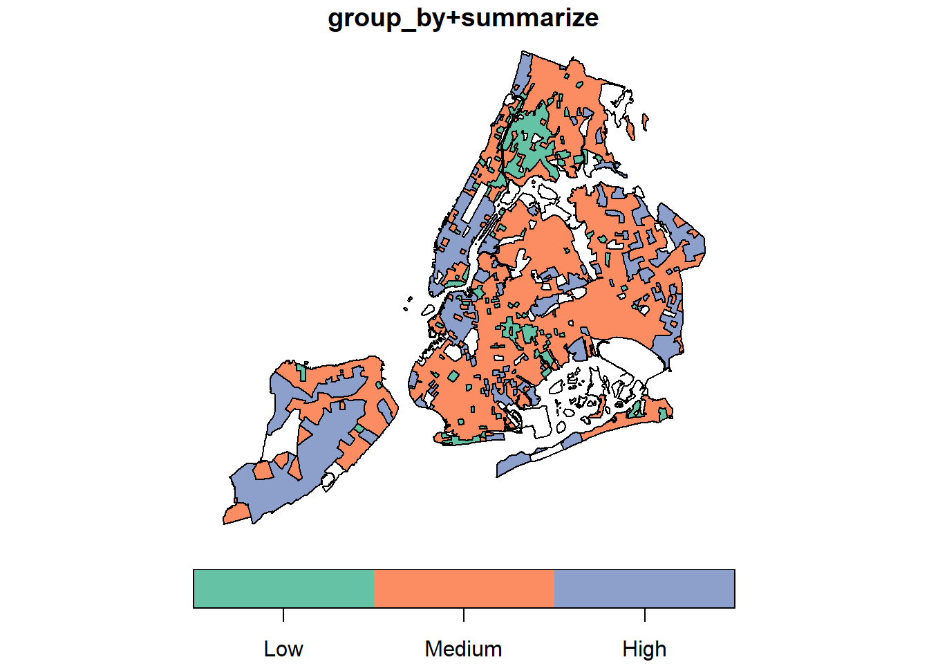
groupFactor <- cut(nyc_sf_merged$MEDHHINC,
c(0, 30000, 80000, Inf),
c('Low', 'Medium', 'High'));
nyc_sf_merged %>%
dplyr::select(MEDHHINC, geometry ) %>%
aggregate(by = list(FemDocLevel = groupFactor), sum) %>%
magrittr::extract('FemDocLevel') %>% plot(main="dissolve by aggregate")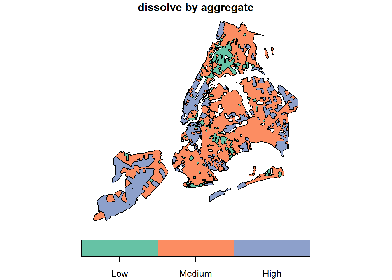
2.7 Lab Assignment
The second lab is to aggregate data from different sources to the zip codes as the core covid-19 data are available at that scale.
Main tasks for the second lab are:
- Join the COVID-19 data to the NYC zip code area data (sf or sp polygons).
- Aggregate the NYC food retails store data (points) to the zip code data, so that we know how many retail stores in each zip code area. Note that not all locations are for food retail. And we need to choose the specific types according to the data.
- Aggregate the NYC health facilities (points) to the zip code data. Similarly, choose appropriate subtypes such as nursing homes from the facilities.
- Join the Census ACS population, race, and age data to the NYC Planning Census Tract Data.
- Aggregate the ACS census data to zip code area data.
In the end, we should have the confirmed and tested cases of covid-19, numbers of specific types of food stores, numbers of specific types of health facilities, and population (total population, elderly, by race, etc.) at the zip code level. We should also have boroughs, names, etc. for each zip code area.
Lovelace, R., Nowosad, J., & Muenchow, J. (2019). Geocomputation with R. CRC Press.↩︎
Per the ESRI specification a Shapefile must have an attribute table, so when we read it into R with the
readOGRcommand from the sp package it automatically becomes aSpatial*Dataframeand the attribute table becomes the data.frame.↩︎