Chapter 1 Introduction to spatial data in R
Learning Objectives
- Understand the structure of sf objects
- Read spatial data into sf objects
- Create sf objects from coordinate columns
- Map sf data with static and interactive visuals
- Read GeoTiff single and multiband into a terraSpatRaster object (optional).
- Examine SpatRaster objects (optional)
1.1 Spatial vector data model in R
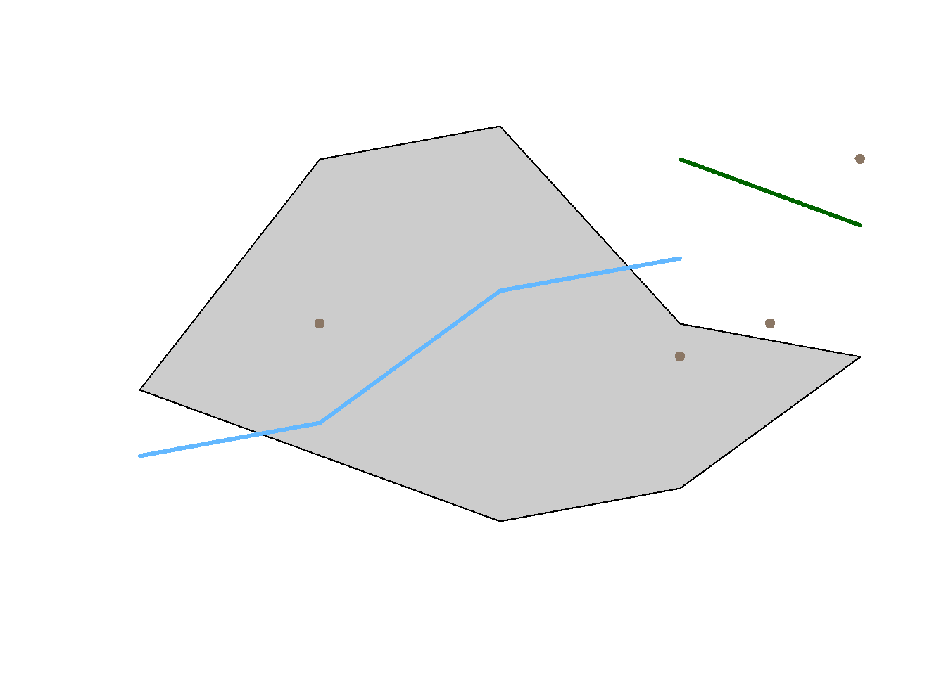
In the vector model of spatial data, we have types of points (Points, MultiPoints), lines (LinesStrings, MultiLineStrings), polygons (Polygons, MultiPolygons), and a combination of them (GeometryCollection).
But these are pure geometries defined in the Euclidean space with Cartesian coordinates. we need to refer such data to physical locations on the Earth surface, aka “geographically referenced.” In order to do that, the software need to know extra information about the shape of the 3D Earth surface and how locations on the 3D surface can be projected or transformed to 2D surfaces like our paper maps and computer screens. The spatial reference systems (SRS) or coordinate reference systems (CRS) are the solution, which have been fully developed in Geographic Information Science or Geographic Information Systems.
- In the next session, we will continue to examine some of the details of CRS. In this session, we start to learn how it is defined and used.
- Geographic data, by definition, are spatial data with reference to the Earth surface. Spatial data, by contrast, could refer to any surfaces or spaces. In other words, all geographic data are spatial data but some spatial data are not geographic data. While mostly interchangeable, they could be usefully differentiated in some contexts.
1.1.1 Handling spatial data in R
Spatial data analysis has always been an important component in the R ecosystem. For vector spatial data in R, there are two families of data structures based on two packages.
- sp family: used to be de facto standard and still popular
- sp means spatial and defines a family of spatial data classes.
- some of the top level classes are SpaitalPointsDataFrame, SpatialMultiPointsDataFrame, SpatialLinesDataFrame, and SpatialPolygonsDataFrame.
- The ESRI Shapefile is closest to sp in terms of data organization.
- sf family: the newer and “modern” standard
- sf means Simple Feature Specification as defined by Open Geospatial Consortium or OGC.
- It is faster, more efficient, and consistent with other software like PostGIS.
- sf is supported by the R Consortium and therefore “official.”
- It is almost the same as the table format in spatial databases like PostGIS and SpatiaLite.
- sf is tidyverse compatible and works well with tidy-packages like dplyr, ggplot, and tidycensus
One must understand that sp and sf are not two rivals in the R ecosystem. Instead, sf is more like a natural evolution of sp. First, there is demand to unify the data models across the entire geospatial industry so that GIS software and spatial databases are compatible and interoperable. OGC is leading the development of such geospatial standards. Most organizations and products like QGIS, PostGIS, Oracle, and ArcGIS are increasingly adopting them. And sf was a response from the R spatial community to these standards.
Second, R now has more advanced data processing features and better fundamental packages such as those in the tidyverse. For geospatial data, more efficient open source spatial libraries also become available based on libraries like RGEOS, GDAL, PROJ, boost geometry etc. The new sf package can better take advantage of these developments.
Practically, it is very easy to convert between sp and sf structures as their underlying spatial models are compatible. And some of the key developers are actually working on both packages. Many R spatial packages can use both. But in case a package can only use one of them, we must make explicit conversions, mostly from sf to sp because most classic R spatial packages are based on sp.
That being said, when and where possible, we should always give the sf-family packages a higher priority as most packages are reworking towards being tidyverse compatible. Some packages related to the sp family packages are retiring. For this course, we focus on the sf package.
1.1.2 The sf package
The sf1 package is first released on CRAN in late October 2016 . It implements a formal standard called “Simple Features” that specifies a storage and access model of spatial geometries such as points, lines, and polygons. A feature geometry is called simple when it meets certain criteria. For example, simple polygons cannot self-intersect and they cannot have spikes or dangling vertexes. Simple Features are independent and have no explicit information about their neighbors or other spatially connected features. This standard has been adopted widely, not only by spatial databases such as PostGIS, but also web standards such as GeoJSON.
If you work with PostGIS or GeoJSON you may have come across the WKT (well-known text) format (Fig 1.1 and 1.2). Note that these texts are not what are being actually saved or encoded in the data. They are just for users’ convenience as they are readable as opposed to the binary code.
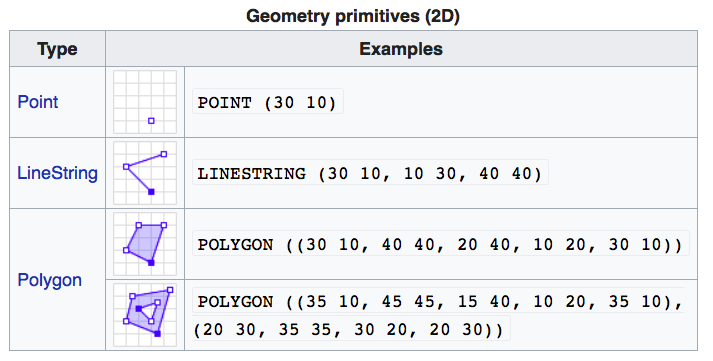
FIGURE 1.1: Well-Known-Text Geometry primitives (wikipedia)
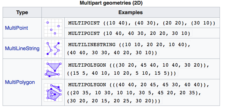
FIGURE 1.2: Well-Known-Text Multipart geometries (wikipedia)
sf implements the Simple Features standard natively in R. sf stores spatial objects as a simple data frame with a special column that contains the information for the geometry coordinates. That special column is a list with the same length as the number of rows in the data frame. Each of the individual list elements then can be of any length needed to hold the coordinates that correspond to an individual feature.
How simple features in R are organized
The three classes used to represent simple features are:
- sf, the table (data.frame) with feature attributes and feature geometries, which contains
- sfc, the list-column with the geometries for each feature (record), which is composed of
- sfg, the feature geometry of an individual simple feature.
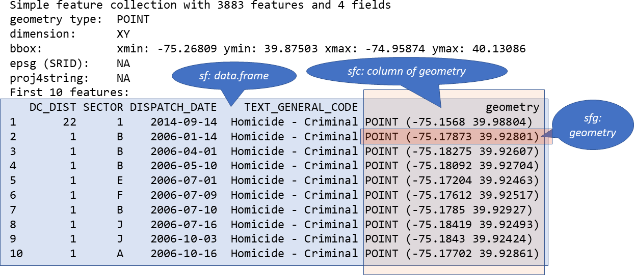
FIGURE 1.3: Relationship of sf, sfc, and sfg
1.1.3 Create a spatial sf object manually
The basic steps of creating sf objects are bottom-up, that is from sfg, to sfc, then to sf.
I. Create geometric objects
Geometric objects (simple features) can be created from a numeric vector, matrix or a list with the coordinates. They are called sfg objects for Simple Feature Geometry. In sf package, there are functions that help create simple feature geometries, like st_point(), st_linestring(), st_polygon() and more.
- Combine all individual single feature objects for the special column.
The feature geometries are then combined into a Simple Feature Collection with st_sfc(). which is nothing other than a simple feature geometry list-column. The sfc object also holds the bounding box and the projection information.
- Add attributes.
Lastly, we add the attributes to the the simple feature collection with the st_sf() function. This function extends the well known data frame in R with a column that holds the simple feature collection.
Here we try to creat some highway objects. First, we would generate LINESTRINGs as simple feature geometries sfg out of a matrix with coordinates:
set.seed(1006) # for replicability
# runif(6) generates 6 random numbers in uniform distribution
lnstr_sfg1 <- st_linestring(matrix(runif(6), ncol=2))
set.seed(1043)
lnstr_sfg2 <- st_linestring(matrix(runif(6), ncol=2))
class(lnstr_sfg1)#> [1] "XY" "LINESTRING" "sfg"We would then combine this into a simple feature collection sfc:
#> [1] "sfc_LINESTRING" "sfc"And lastly use our data frame from above to generate the sf object:
dfr <- data.frame(id = c("hwy1", "hwy2"), cars_per_hour = c(78, 22))
lnstr_sf <- st_sf(dfr , lnstr_sfc)
class(lnstr_sf)#> [1] "sf" "data.frame"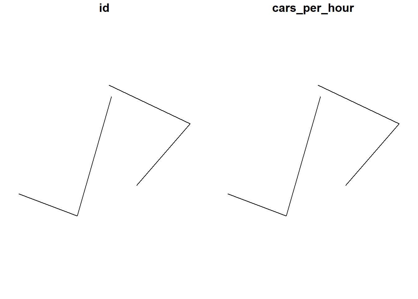
1.1.4 sf methods
There are many methods available in the sf package. Most function names, particularly those related to spatial data processing and analysis, start with st_, which means Spatial Type. To find out more, use
#> [1] $<- [
#> [3] [[<- [<-
#> [5] aggregate anti_join
#> [7] arrange as.data.frame
#> [9] cbind coerce
#> [11] crs dbDataType
#> [13] dbWriteTable distance
#> [15] distinct dplyr_reconstruct
#> [17] drop_na duplicated
#> [19] ext extract
#> [21] filter full_join
#> [23] gather group_by
#> [25] group_split identify
#> [27] initialize inner_join
#> [29] left_join lines
#> [31] mapView mask
#> [33] merge mutate
#> [35] nest pivot_longer
#> [37] pivot_wider plot
#> [39] points polys
#> [41] print rasterize
#> [43] rbind rename
#> [45] rename_with right_join
#> [47] rowwise sample_frac
#> [49] sample_n select
#> [51] semi_join separate
#> [53] separate_rows show
#> [55] slice slotsFromS3
#> [57] spread st_agr
#> [59] st_agr<- st_area
#> [61] st_as_s2 st_as_sf
#> [63] st_as_sfc st_bbox
#> [65] st_boundary st_break_antimeridian
#> [67] st_buffer st_cast
#> [69] st_centroid st_collection_extract
#> [71] st_concave_hull st_convex_hull
#> [73] st_coordinates st_crop
#> [75] st_crs st_crs<-
#> [77] st_difference st_drop_geometry
#> [79] st_exterior_ring st_filter
#> [81] st_geometry st_geometry<-
#> [83] st_inscribed_circle st_interpolate_aw
#> [85] st_intersection st_intersects
#> [87] st_is st_is_full
#> [89] st_is_valid st_join
#> [91] st_line_merge st_m_range
#> [93] st_make_valid st_minimum_bounding_circle
#> [95] st_minimum_rotated_rectangle st_nearest_points
#> [97] st_node st_normalize
#> [99] st_point_on_surface st_polygonize
#> [101] st_precision st_reverse
#> [103] st_sample st_segmentize
#> [105] st_set_precision st_shift_longitude
#> [107] st_simplify st_snap
#> [109] st_sym_difference st_transform
#> [111] st_triangulate st_triangulate_constrained
#> [113] st_union st_voronoi
#> [115] st_wrap_dateline st_write
#> [117] st_z_range st_zm
#> [119] summarise svc
#> [121] text transform
#> [123] transmute ungroup
#> [125] unite unnest
#> [127] vect
#> see '?methods' for accessing help and source codeHere are some of the other highlights of sf that you might be interested in:
provides fast I/O, particularly relevant for large files
spatial functions that rely on GEOS and GDAL and PROJ external libraries are directly linked into the package, so no need to load additional external packages (like in sp)
sf objects can be plotted directly with
ggplotsf directly reads from and writes to spatial databases such as PostGIS
sf is compatible with the
tidyvderse, (but see some pitfalls here)
Note that sp and sf are not the only way spatial objects are conceptualized in R. Other spatial packages may use their own class definitions for spatial data (for example spatstat).
There are packages specifically for the GeoJSON and for that reason are more lightweight, for example:
Usually you can find functions that convert objects to and from these formats.
Self-Exercise
Similarly to the example above generate a Point object in R.
- Create a matrix pts of random numbers with two columns and as many rows as you like. These are your points.
- Create a dataframe attrib_df with the same number of rows as your pts matrix and a column that holds an attribute. You can make up any attribute.
- Use the appropriate commands and pts to create an sf object with a geometry column of class sfc_POINT.
- Try to subset/filter your spatial object using the attribute you have added and the way you are used to from regular data frames.
- How do you determine the bounding box of your spatial object?
1.2 Load and Display Data with sf
With good understanding of the sf data structure, we are ready to load and display some real data.
1.2.1 Reading Shapefiles into R
sf utilizes the powerful GDAL library to conduct data I/O (input/output), which is automatically loaded when loading sf. GDAL can handle numerous vector and raster data format. The st_read() method in sf is the interface for reading vector spatial data. In this section, we mostly use the Shapefile format.
# read in a Shapefile. With the 'shp' file extension, sf knows it is a Shapefile.
nyc_sf <- st_read("data/nyc/nyc_acs_tracts.shp")#> Reading layer `nyc_acs_tracts' from data source
#> `D:\Cloud_Drive\Hunter College Dropbox\Shipeng Sun\Workspace\RSpace\R-Spatial_Book\data\nyc\nyc_acs_tracts.shp'
#> using driver `ESRI Shapefile'
#> Simple feature collection with 2166 features and 113 fields
#> Geometry type: MULTIPOLYGON
#> Dimension: XY
#> Bounding box: xmin: -74.25559 ymin: 40.49612 xmax: -73.70001 ymax: 40.91553
#> Geodetic CRS: NAD83# take a look at what we've got
str(nyc_sf) # note again the geometry column at the end of the output#> Classes 'sf' and 'data.frame': 2166 obs. of 114 variables:
#> $ UNEMP_RATE: num 0 0.0817 0.1706 0 0.088 ...
#> $ cartodb_id: num 1 2 3 4 5 6 7 8 9 10 ...
#> $ withssi : int 0 228 658 0 736 0 261 0 39 638 ...
#> $ withsocial: int 0 353 1577 0 1382 99 1122 10 264 895 ...
#> $ withpubass: int 0 47 198 0 194 0 145 0 5 334 ...
#> $ struggling: int 0 694 2589 0 2953 337 3085 17 131 1938 ...
#> $ profession: int 0 0 36 0 19 745 18 49 35 0 ...
#> $ popunemplo: int 0 92 549 0 379 321 432 26 106 494 ...
#> $ poptot : int 0 2773 8339 0 10760 7024 10955 849 1701 5923 ...
#> $ popover18 : int 0 2351 6878 0 8867 6637 8932 711 1241 4755 ...
#> $ popinlabou: int 0 1126 3218 0 4305 5702 5114 657 735 2283 ...
#> $ poororstru: int 0 2026 4833 0 7044 1041 6376 112 232 4115 ...
#> $ poor : int 0 1332 2244 0 4091 704 3291 95 101 2177 ...
#> $ pacificune: int 0 0 0 0 13 0 0 0 0 0 ...
#> $ pacificinl: int 0 0 0 0 13 0 0 0 0 0 ...
#> $ pacific : int 0 0 0 0 13 0 0 0 0 0 ...
#> $ otherunemp: int 0 0 103 0 46 0 0 0 17 151 ...
#> $ otherinlab: int 0 144 348 0 609 112 184 48 90 525 ...
#> $ otherethni: int 0 598 1175 0 1799 112 377 48 183 1664 ...
#> $ onlyprofes: int 0 0 102 0 20 890 116 78 77 0 ...
#> $ onlymaster: int 0 77 412 0 292 2162 408 233 328 16 ...
#> $ onlylessth: int 0 878 2164 0 3793 121 4384 34 115 1846 ...
#> $ onlyhighsc: int 0 1088 4068 0 3868 5508 3882 631 1093 2343 ...
#> $ onlydoctor: int 0 0 66 0 1 145 98 29 42 0 ...
#> $ onlycolleg: int 0 471 2355 0 2290 5371 2223 585 884 1111 ...
#> $ onlybachel: int 0 271 1269 0 1322 4685 1262 481 687 200 ...
#> $ okay : int 0 742 3474 0 3499 5982 4579 733 1469 1798 ...
#> $ mixedunemp: int 0 16 21 0 14 24 0 0 51 31 ...
#> $ mixedinlab: int 0 72 134 0 100 136 91 10 62 140 ...
#> $ mixed : int 0 175 234 0 251 224 115 16 102 334 ...
#> $ master : int 0 77 310 0 272 1272 292 155 251 16 ...
#> $ maleunempl: int 0 76 349 0 179 204 197 8 72 277 ...
#> $ maleover18: int 0 1101 3134 0 4068 3557 3992 454 613 1935 ...
#> $ malepro : int 0 0 36 0 19 473 48 51 61 0 ...
#> $ malemastr : int 0 10 143 0 126 1034 181 123 139 0 ...
#> $ male_lesHS: int 0 302 1063 0 1693 29 2013 17 103 714 ...
#> $ male_HS : int 0 607 1893 0 1651 2985 1702 414 485 985 ...
#> $ male_doctr: int 0 0 24 0 0 77 30 29 38 0 ...
#> $ male_collg: int 0 227 1225 0 997 2924 871 381 368 462 ...
#> $ male_BA : int 0 132 668 0 562 2411 499 288 292 43 ...
#> $ maleinlabo: int 0 612 1640 0 2059 3299 2466 423 392 991 ...
#> $ maledrop : int 0 16 8 0 0 0 0 0 0 0 ...
#> $ male16to19: int 0 65 253 0 162 37 236 20 32 187 ...
#> $ male : int 0 1318 3850 0 4796 3840 5244 533 897 2514 ...
#> $ lessthanhi: int 0 878 2164 0 3793 121 4384 34 115 1846 ...
#> $ lessthan10: int 0 212 760 0 1100 289 625 2 51 463 ...
#> $ households: int 0 986 3382 0 3838 4104 3950 367 739 2224 ...
#> $ hispanicun: int 0 30 269 0 115 27 0 0 68 335 ...
#> $ hispanicin: int 0 357 1171 0 819 297 236 77 201 1145 ...
#> $ hispanic : int 0 1187 3503 0 2608 374 318 108 360 3478 ...
#> $ highschool: int 0 617 1713 0 1578 137 1659 46 209 1232 ...
#> $ geo_state : int 36 36 36 36 36 36 36 36 36 36 ...
#> $ geo_place : int 51000 51000 51000 51000 51000 51000 51000 51000 51000 51000 ...
#> $ geo_county: int 61 61 61 61 61 61 61 61 61 61 ...
#> $ field_1 : int 1 2 3 4 5 6 7 8 9 10 ...
#> $ femaleunem: int 0 16 200 0 200 117 235 18 34 217 ...
#> $ femaleover: int 0 1250 3744 0 4799 3080 4940 257 628 2820 ...
#> $ fem_profes: int 0 0 66 0 1 417 68 27 16 0 ...
#> $ fem_master: int 0 67 269 0 166 1128 227 110 189 16 ...
#> $ fem_lessHS: int 0 576 1101 0 2100 92 2371 17 12 1132 ...
#> $ fem_HS : int 0 481 2175 0 2217 2523 2180 217 608 1358 ...
#> $ fem_doctor: int 0 0 42 0 1 68 68 0 4 0 ...
#> $ fem_colleg: int 0 244 1130 0 1293 2447 1352 204 516 649 ...
#> $ fem_BA : int 0 139 601 0 760 2274 763 193 395 157 ...
#> $ femaleinla: int 0 514 1578 0 2246 2403 2648 234 343 1292 ...
#> $ femaledrop: int 0 0 1 0 0 0 0 0 0 14 ...
#> $ femal16_19: int 0 84 124 0 271 2 126 2 32 242 ...
#> $ female : int 0 1455 4489 0 5964 3184 5711 316 804 3409 ...
#> $ europeanun: int 0 14 328 0 56 188 71 26 22 132 ...
#> $ europeanin: int 0 303 1641 0 525 4058 492 540 543 510 ...
#> $ european : int 0 540 4091 0 1181 4975 929 717 1327 1645 ...
#> $ doctorate : int 0 0 66 0 1 145 98 29 42 0 ...
#> $ com_90plus: int 0 49 101 0 36 61 82 17 27 178 ...
#> $ comm_5less: int 0 99 0 0 1 220 46 26 0 0 ...
#> $ comm_60_89: int 0 40 215 0 370 136 687 32 41 331 ...
#> $ comm_5_14 : int 0 121 226 0 331 913 718 87 58 99 ...
#> $ comm_45_59: int 0 142 171 0 284 287 409 46 84 351 ...
#> $ comm_30_44: int 0 217 923 0 1442 1514 1118 198 210 493 ...
#> $ comm_15_29: int 0 352 970 0 1250 1840 1363 192 134 304 ...
#> $ college : int 0 200 1086 0 968 686 961 104 197 911 ...
#> $ bachelor : int 0 194 857 0 1030 2523 854 248 359 184 ...
#> $ asianunemp: int 0 62 38 0 207 108 352 0 16 61 ...
#> $ asianinlab: int 0 559 615 0 2736 1286 4283 42 35 491 ...
#> $ asian : int 0 1249 1724 0 6549 1598 9448 51 75 922 ...
#> $ americanun: int 0 0 0 0 0 1 0 0 0 24 ...
#> $ americanin: int 0 0 0 0 57 1 0 0 0 24 ...
#> $ american : int 0 43 0 0 57 1 0 0 0 51 ...
#> $ africanune: int 0 0 59 0 43 0 9 0 0 95 ...
#> $ africaninl: int 0 48 434 0 265 109 64 17 5 593 ...
#> $ african : int 0 168 1115 0 910 114 86 17 14 1307 ...
#> $ puma : chr "3810" "3809" "3809" "3810" ...
#> $ ntaname : chr "park-cemetery-etc-Manhattan" "Lower East Side" "Lower East Side" "park-cemetery-etc-Manhattan" ...
#> $ ntacode : chr "MN99" "MN28" "MN28" "MN99" ...
#> $ ctlabel : chr "1" "2.01" "2.02" "5" ...
#> $ cdeligibil: chr "I" "E" "E" "I" ...
#> $ boroname : chr "Manhattan" "Manhattan" "Manhattan" "Manhattan" ...
#> $ medianinco: num NA 17282 24371 NA 18832 ...
#> $ medianagem: num NA 39.3 44.9 NA 43.4 29.7 42 33.2 41.5 31.2 ...
#> $ medianagef: num NA 43.8 47.9 NA 43 28.3 43 31.9 45.7 47.5 ...
#> [list output truncated]
#> - attr(*, "sf_column")= chr "geometry"
#> - attr(*, "agr")= Factor w/ 3 levels "constant","aggregate",..: NA NA NA NA NA NA NA NA NA NA ...
#> ..- attr(*, "names")= chr [1:113] "UNEMP_RATE" "cartodb_id" "withssi" "withsocial" ...Two more words about the geometry column: The geometry column does not have to be named “geometry”. You can name this column any way you wish. “geom”, for example, is another popular name for the geometry column. Secondly, you can remove this column and revert to a regular, non-spatial dataframe at any time with st_drop_geometry().
1.2.2 Simple sf plotting
The default plot of an sf object is a multi-plot of the first attributes, with a warning if not all can be plotted. By default, it plots the first 9 columns:
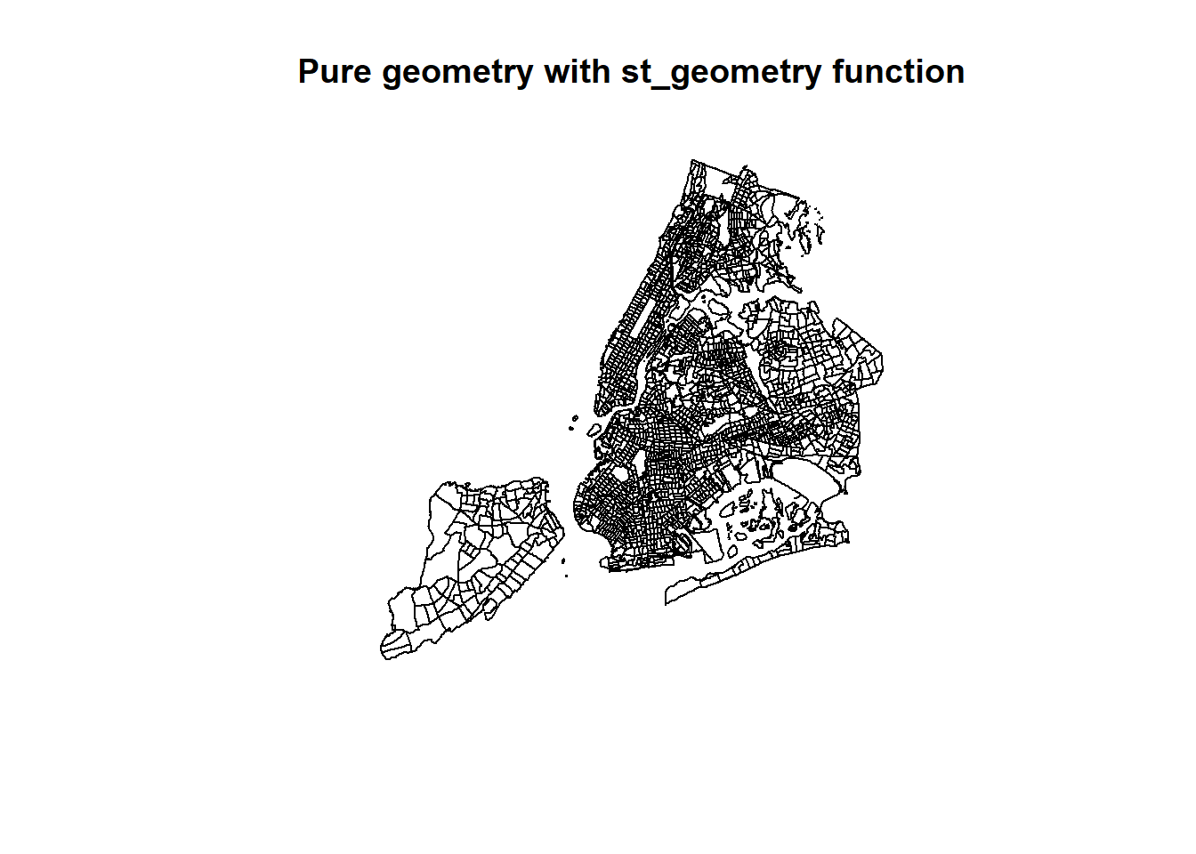
In order to only plot the polygon boundaries we need to directly use the geometry column. We use the st_geometry() function to extract it. We can also select a single column or a few columns to draw.
# Only the college column, with geometry
plot(nyc_sf['college'], main='One column with ["college"]')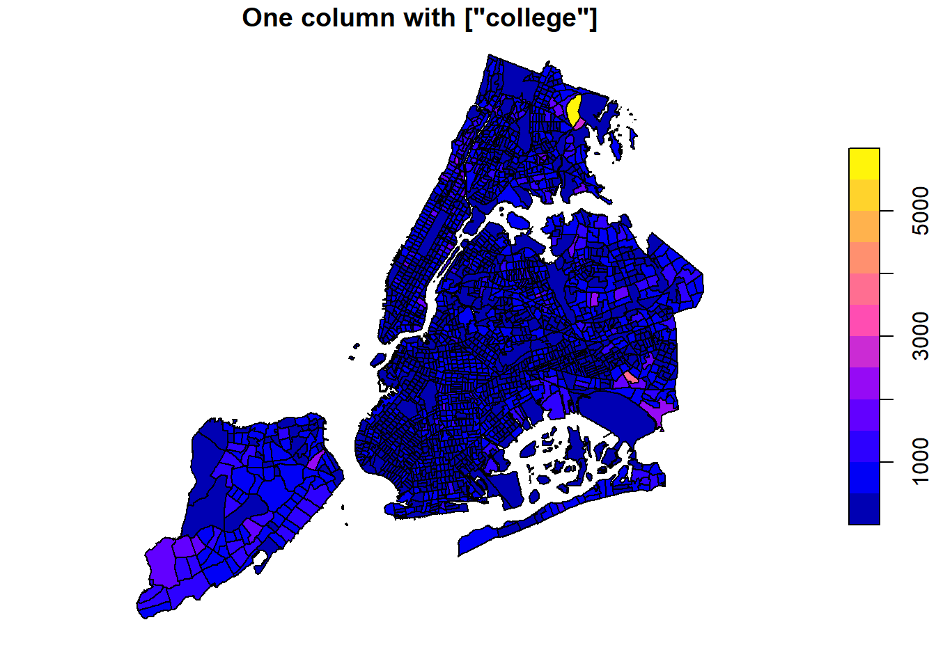
# Two columns, with geometry
plot(nyc_sf[c('college', 'fem_colleg')], main='Two Columns with ["college", "fem_colleg"]')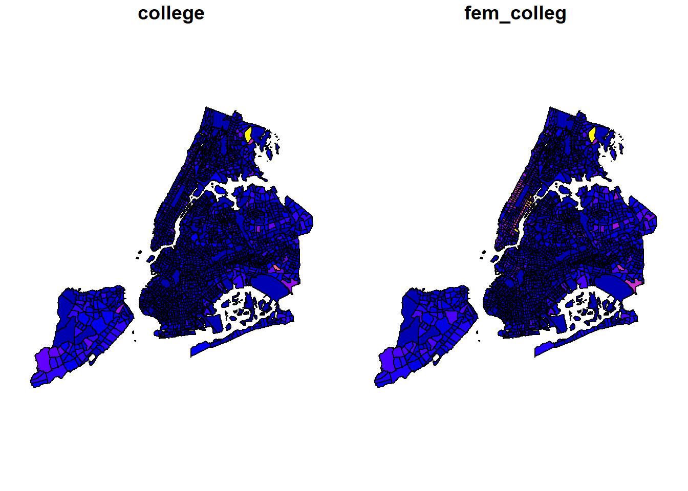
Let’s add a subset of polygons with only the census tracts where the median household income is more than $80,000. We can extract elements from an sf object based on attributes using your preferred method of filtering dataframes.
# Make a plot using all tracts, then add the "rich" in red
plot(st_geometry(nyc_sf))
plot(st_geometry(nyc_sf_rich), add=T, col="red")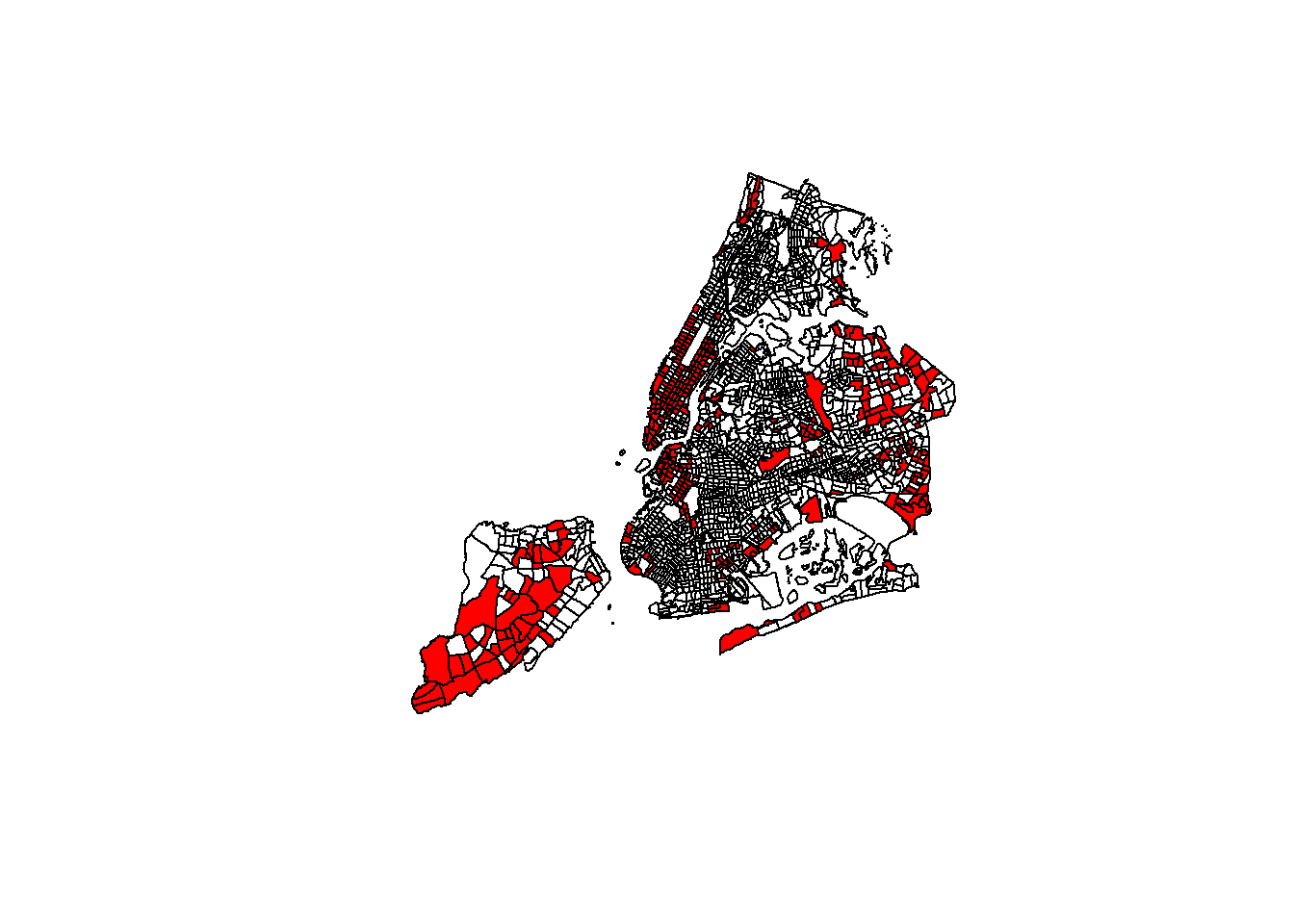
tidyverse and piping work as well!
1.2.3 Simple interactive mapping with mapview
One of most useful, yet simplest methods of visualizing a sf object or other spatial data is to utilize the mapview package for interactive mapping. mapview utilizes the leaflet package in R and the original JavaScript leaflet library for web mapping. While we will learn the details of leaflet later, here is a quick application of the mapview package.
# We use all the default options, but select a few columns.
# If we use all columns, the popup window will be too big.
nyc_sf %>% dplyr::select(boroname, poptot, female, doctorate) %>%
mapview::mapview()Further configuration could be applied.
nyc_sf %>% dplyr::select(boroname, poptot, female, doctorate) -> tmp_sf
mapview(tmp_sf, zcol='boroname', layer.name = 'Borough', stroke=FALSE) +
mapview(tmp_sf, zcol='poptot',
layer.name = 'Total Population',
homebutton=FALSE,
legend=FALSE,
hide = TRUE) +
mapview(tmp_sf, zcol="doctorate",
layer.name = 'Population with Doctorate',
homebutton=FALSE,
legend=FALSE,
hide=TRUE,
label="doctorate",
popup = 'doctorate')