Lab 12
Bivariate
Statistics
This lab
exercise corresponds directly with the lecture by the same name. By now, you
are familiar with the format of ![]() exercises. After a brief repeat of the
concept, a short example of its application in
exercises. After a brief repeat of the
concept, a short example of its application in ![]() is given and where applicable particular
idiosyncrasies (oddities) of
is given and where applicable particular
idiosyncrasies (oddities) of ![]() reported. This is followed up with a lab
question, where you are to apply to concepts learned. In this lab, we have four
steps covering four related topics. There is a brief question incorporated into
each of these four steps.
reported. This is followed up with a lab
question, where you are to apply to concepts learned. In this lab, we have four
steps covering four related topics. There is a brief question incorporated into
each of these four steps.
Step 1 Two-sample difference of means test
Geographers
use two primary methods to compare and test means from two independent samples
for significance of difference. If the sample data and population distributions
meet the requirements the appropriate independent sample difference of means
procedure would be the t test. In this case, the sample data
would have to be measured on the interval or ratio scale and the samples must be
drawn from normally distributed populations. Conversely, if the sample data are
measured at the ordinal or nominal scale, a non-parametric procedure is
required. The Wilcoxon rank sum W test is most commonly used. We discussed the t
test in the previous lab and will therefore concentrate here on
the non-parametric tests. Be it just mentioned here that instead of comparing a
sample to a population or an expected value, we now compare it with a second
sample.
Rather
than using parameters like mean and variance, non-parametric techniques use the
ranks of sample observations to
measure the magnitude of the differences in ranked positions between the two
sets of sample data. The Wilcoxon test uses a
variation of the t test to see if the sum of sample ranks
is significantly different from what it should be if the two samples are
actually drawn from the same population. The test statistic W for the two-sample Wilcoxon
procedure is
![]()
where ![]() is the mean rank
is the mean rank ![]() with nS
being the small and nB
the bigger sample.
with nS
being the small and nB
the bigger sample.
The
similarity in philosophy between the t
and the Wilcoxon W
tests is mirrored by their use in ![]() . The airquality data set built into
. The airquality data set built into ![]() lists among other things ozone readings for
the months May through September. List the contents of the airquality data set, plot it by month, and
then run the t and W statistics.
lists among other things ozone readings for
the months May through September. List the contents of the airquality data set, plot it by month, and
then run the t and W statistics.
> airquality
>
boxplot (Ozone ~ Month, data
= airquality)
# notice the use of the ~ tilde operator to specify that Ozone is described by Month
> t.test(Ozone ~ Month, data = airquality, subset = Month %in% c(5, 8))
> wilcox.test(Ozone ~ Month, data = airquality,
subset = Month %in% c(5, 8))
Now you will
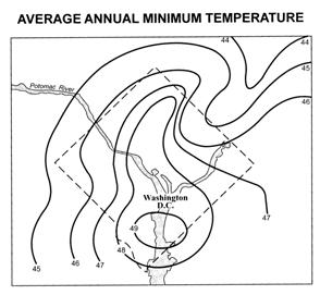
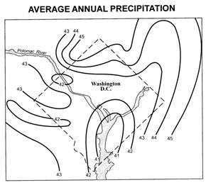
conduct a similar analysis on urban microclimates. It is widely recognized that
climate characteristics in cities differ considerably from those in the
surrounding country-side. In “The Climate of Cities” (Scientific American, 217:15-23),
William Lowry (1967) discusses the basic influences that set a city’s climate
apart from that of the surrounding area. The washclim dataset has been derived from this article and will serve
you to determine whether temperature and precipitation differ significantly
between the city and countryside in the
|
|
|
![]() 1 Have
a look at the washclim data set and
1 Have
a look at the washclim data set and
(a) determine what are the dependent and what are the independent variables,
(b) describe in plain English the two null hypotheses H0.
![]() 2 Use
the washclim data set
to
2 Use
the washclim data set
to
(a) conduct a difference of means t test with the
interval/ratio based data, and
(b) apply the Wilcoxon rank sum test to the same
dataset after you downgraded it to an ordinal scale.
Both the t
and the Wilcoxon test require the two samples
to be independent from each other. If this requirement is not met, a matched-pairs difference test is in
order.
Step 2 Dependent sample difference test
Geographers
often want to determine if two sets of values defined for one group of
individuals or spatial locations differ. For examples, suppose one wishes to
compare the number of migrants moving into a set of counties with the number of
migrants leaving the same set of counties. While at first sight, a difference
of means t or Wilcoxon rank
sum W
may seem appropriate, these tests do not qualify because they require independent samples. The dependent
sample difference test measures the differences within matched pairs of
observations. As before, we separate a matched-pair t test for ration or interval
data from the Wilcoxon matched-pairs signed ranks
test for ordinal or non-parametric data.
The null
hypothesis in the matched-pairs problem states that the mean difference for all
matched pairs, ![]() ,
in the population equals zero. The test statistic
,
in the population equals zero. The test statistic ![]() is
calculated analogous to the regular t test (mp stands for matched-pair and d for difference). If the difference is
non-zero but small, we will not reject this null hypothesis. The challenge now
lies in figuring out what difference is big enough to suggest that the two
samples do indeed come from different sub populations rather than one
homogenous one. As usual, this can only be answered by the domain scientist and
not the statistician. The Wilcoxon matched-pairs
signed ranks test statistic looks frightening but is actually quite simple and
again analogous to the one based on independent samples:
is
calculated analogous to the regular t test (mp stands for matched-pair and d for difference). If the difference is
non-zero but small, we will not reject this null hypothesis. The challenge now
lies in figuring out what difference is big enough to suggest that the two
samples do indeed come from different sub populations rather than one
homogenous one. As usual, this can only be answered by the domain scientist and
not the statistician. The Wilcoxon matched-pairs
signed ranks test statistic looks frightening but is actually quite simple and
again analogous to the one based on independent samples:

Let’s look
at a geographic example. Global warming has been recognized as one of the most severe
threats to life on this planet as we know it. A way to test for global warming
would be to record temperatures at a single set of locations over a time
period. Because this problem uses only one variable collected at two different
time periods, a matched-pair or dependent sample difference test is most
appropriate. The corntemp dataset consists of a sample of 28
weather stations located within the American Corn Belt with the average annual
temperature calculated for a two-year period in the mid-1970’s and in the
mid-1990’s. Of the 28 stations, 18 showed warmer average temperatures over the
20-yeaer period, 7 showed colder averages, and 3 stations showed no change.
Over all 28 stations, the temperature rose on average 0.2 degrees Celsius.
![]() 3 Use
the corntemp dataset to
calculate the likelihood of committing a Type I error. How (statistically)
confident are you in your judgment?
3 Use
the corntemp dataset to
calculate the likelihood of committing a Type I error. How (statistically)
confident are you in your judgment?
You would want to calculate the average difference, the standard error of that
difference, the tmp
statistic and a (one-tailed) p value.
Step 3 Chi-square goodness-of-fit test
Depending
on the circumstances, a set of data can be tested for “fit” against a variety
of expected, sometimes theoretical frequency distributions. The expected
frequency distribution would for example be the uniform one, if we were to
examine nutrient runoff levels from a series of adjacent agricultural land use
tributaries running into the same bay. If, on the other hand, we know that the
distribution of farmland among the five tributaries varies widely, then we
might want to hypothesize a distribution that is proportional to the amount of
farmland in each watershed. Again, we distinguish between cases of interval/ratio
data on one side and ordinal or nominal data on the other. This time, we start
with the latter, and the appropriate test is known as the Chi-square (c2) Goodness-of-Fit test.
When
applied as a goodness-of-fit test, the chi-square statistic compares observed
frequency counts of a single variable with an expected distribution of frequency counts. The null hypothesis
states that the population from which the sample is drawn fits an expected distribution;
thus there is no difference between observed and expected frequency counts. The
formula for the chi-square test statistic is

With k = number of nominal or ordinal
categories.
Example:
A newly appointed school district superintendent wants to
conduct a geographic study that compares SAT test scores among graduating
seniors from five comparably sized high schools in different parts of
|
John Muir |
Gifford Pinchot |
Rachel Carson |
Garrett Hardin |
Aldo Leopold |
|
42 |
45 |
51 |
47 |
60 |
Ei = SOi / k = 245/5 = 49
c2 = (42-49)2/49 + (45-49)2/49 +
(51-49)2/49 + (47-49)2/49 +
(60-49)2/49 = 3.959, and hence p = .412
This is
not a particularly conclusive result – but then, this is what we often get with
real data.
Now it is
your turn to apply the chisq.test() function in ![]() .
.
![]() 4 In
747 cases of “Rocky Mountain spotted fever” from the western
4 In
747 cases of “Rocky Mountain spotted fever” from the western
Step 4 Kolmogorov-Smirnov goodness-of-fit test
For
nominal or ordinal data, we can just list the expected values and compare them
with the observed ones. For interval or ratio data, we rather compare our
observed sample values with those of an expected frequency distribution such as
Poisson or Normal distribution. The Kolmogorov-Smirnov
Goodness-of-Fit test is commonly used by geographers (and others) to test for
normality. More specifically, the Kolmogorov-Smirnov
test compares the cumulative relative
frequencies of the observed sample data with the cumulative frequencies
expected for a perfectly normal distribution. To calculate an observed
cumulative frequency distribution, individual data are ranked from low to high
and then the absolute maximum difference is calculated between the observed and
the expected value based on one distribution or another. For instance, in a
previous lab exercise, you were asked to visually check whether the BWI
precipitation data is normally distributed. You can (and will) do this now with
the Kolmogorov-Smirnov test.
The Kolmogorov-Smirnov test is implemented in ![]() as ks.test(). The first parameter is always the
sample data set. If the second parameter is numeric, a two-sample test of the
null hypothesis that both samples were drawn from the same continuous
distribution is performed. Alternatively, the second parameter can be a
character string naming a continuous distribution function. In this case, a one-sample test is carried
out of the null that the distribution function which generated the sample is
distribution 'xyz'.
as ks.test(). The first parameter is always the
sample data set. If the second parameter is numeric, a two-sample test of the
null hypothesis that both samples were drawn from the same continuous
distribution is performed. Alternatively, the second parameter can be a
character string naming a continuous distribution function. In this case, a one-sample test is carried
out of the null that the distribution function which generated the sample is
distribution 'xyz'.
![]() 5 Read
the BWI data that you know so well by now and use the K-S test to check whether
the data is indeed normally distributed.
5 Read
the BWI data that you know so well by now and use the K-S test to check whether
the data is indeed normally distributed.
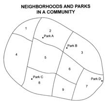
With this, we covered all the material for this lab
exercise. Let’s now apply the c2 test in a real geographic problem setting. An intermediate-sized
community contains four city parks and nine identifiable neighborhoods (see map
below). Members of the city park and recreation department have been collecting
information on park usage by neighborhood. The following visitation data have
been collected:
|
|
Neighborhood |
||||||||
|
Park ID
and Name |
1 |
2 |
3 |
4 |
5 |
6 |
7 |
8 |
9 |
|
A: |
120 |
312 |
110 |
76 |
195 |
62 |
58 |
62 |
52 |
|
B: |
70 |
110 |
410 |
53 |
82 |
101 |
80 |
60 |
78 |
|
C: |
60 |
62 |
61 |
94 |
114 |
85 |
74 |
280 |
96 |
|
D: |
35 |
40 |
110 |
38 |
55 |
98 |
512 |
42 |
82 |
![]() 6a For each of the four parks use a chi-square goodness-of-fit test
to determine whether the number of visitors to the park from the nine
neighborhoods is uniformly distributed. Record the p-values for visitations to each of the four parks.
6a For each of the four parks use a chi-square goodness-of-fit test
to determine whether the number of visitors to the park from the nine
neighborhoods is uniformly distributed. Record the p-values for visitations to each of the four parks.
On further
consideration, the community recreation planners suspect that some form of
spatial interaction model might provide a more valid prediction of attendance
at the four city parks. To estimate the number of visitors from each
neighborhood, a simple potential model is applied that hypothesizes park
attendance as being directly related to neighborhood population size and
inversely related to distance from the centroid of
the neighborhood to the park.
![]()
Using this model, the expected number of visitors to each
park from each neighborhood is calculated:
|
|
Neighborhood |
||||||||
|
Park ID
and Name |
1 |
2 |
3 |
4 |
5 |
6 |
7 |
8 |
9 |
|
A: |
106 |
370 |
98 |
71 |
179 |
62 |
50 |
57 |
54 |
|
B: |
68 |
122 |
414 |
47 |
71 |
96 |
81 |
55 |
90 |
|
C: |
52 |
55 |
58 |
80 |
126 |
91 |
71 |
296 |
97 |
|
D: |
34 |
38 |
116 |
44 |
50 |
97 |
507 |
48 |
78 |
![]() 6b For each of the four parks use the data from the table of expected
number of visitors from each neighborhood and apply chi-square as a
goodness-of-fit test to determine whether the number of visitors to the park
from the nine neighborhoods is proportionally distributed as predicted by the
spatial interaction model. Record the p-values
for visitations to each of the four parks.
6b For each of the four parks use the data from the table of expected
number of visitors from each neighborhood and apply chi-square as a
goodness-of-fit test to determine whether the number of visitors to the park
from the nine neighborhoods is proportionally distributed as predicted by the
spatial interaction model. Record the p-values
for visitations to each of the four parks.
Hint: You would make your life easier if you read the observed vs. the expected
values into a matrix of nine values to a row describing a neighborhood.
Record all
your answers to the above six questions and send them in an ASCII email message
to Jing Li.