Lab 08
Introduction to ![]()
This lab
exercise is supposed to help you familiarize yourself with the software
environment that ![]() is. By software environment rather than just
calling it a program, we mean that
is. By software environment rather than just
calling it a program, we mean that ![]() is both a typical application program such as
MS Excel or ArcGIS, as well as a programming environment. With the introduction
to
is both a typical application program such as
MS Excel or ArcGIS, as well as a programming environment. With the introduction
to ![]() ,
we almost sneakingly also introduce you to
programming per se – although this is only a side effect.
,
we almost sneakingly also introduce you to
programming per se – although this is only a side effect.
We recommend
that you have at least three program running concurrently: the web browser to
read this set of instructions, ![]() ,
and a text editor such as Word, WordPad, or something similar. There are no
subdivisions to this lab as you may have gotten used to from the ArcGIS lab.
Mostly, you are just supposed to follow the examples and play with variations
of these.
,
and a text editor such as Word, WordPad, or something similar. There are no
subdivisions to this lab as you may have gotten used to from the ArcGIS lab.
Mostly, you are just supposed to follow the examples and play with variations
of these.
Estimated
time to complete this lab: 90 minutes
Step 1 Start ![]()
If this is
the first time you are using ![]() ,
go to the Windows Start menu, All Programs, R and elect
,
go to the Windows Start menu, All Programs, R and elect ![]() R 2.0.1. After a few seconds, you should see
the following screen:
R 2.0.1. After a few seconds, you should see
the following screen:
Step 1: The R start window.
To
abbreviate this startup sequence, I recommend that you create a shortcut to ![]() either on your desktop or your Quick Launch
taskbar.
either on your desktop or your Quick Launch
taskbar.
Step 2 Know how to get help
No, this
is not about approaching Jing Li for help. ![]() has a number of
built-in ways to get help. One option is the Help menu in the top part of the
has a number of
built-in ways to get help. One option is the Help menu in the top part of the ![]() RGui window. Html
help brings up the same html help pages as the command line
RGui window. Html
help brings up the same html help pages as the command line
> help.start()
You could
also search the help pages for a particular topic through the menu item in the
Help menu, or if you know the command you want to use but not all its
parameters, you can learn about all the details by entering
> help(command)
Now let’s look
at some of the other menu in the RGui.
Step 3 Packages
As you
recall from the lectures, ![]() is a public domain package that consists of
many modules, which here are called packages. By default, that is without you
having to do anything,
is a public domain package that consists of
many modules, which here are called packages. By default, that is without you
having to do anything, ![]() starts with a base package, which as the name
suggests contains a basic set of functionalities and some sample datasets. Also
by default, there are many more packages already installed on your hard disk.
You can see them by picking Load package… from the Packages menu.
starts with a base package, which as the name
suggests contains a basic set of functionalities and some sample datasets. Also
by default, there are many more packages already installed on your hard disk.
You can see them by picking Load package… from the Packages menu.
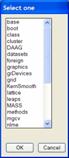
Step 3: Packages already installed
but not yet loaded into memory.
Step 4 Installing additional packages (you
cannot do this on the lab computers!)
If you
downloaded ![]() from one of the Comprehensive R Archive Network
(CRAN) sites to install it on your home computer (something, I, Jochen, highly
recommend you to do), then you can also install additional packages that are
not part of a standard installation. There are literally hundreds of add-on
packages out there. One of the real benefits of
from one of the Comprehensive R Archive Network
(CRAN) sites to install it on your home computer (something, I, Jochen, highly
recommend you to do), then you can also install additional packages that are
not part of a standard installation. There are literally hundreds of add-on
packages out there. One of the real benefits of ![]() is that there are more spatial (geographic)
functions in these public domain packages than in any commercial statistics
software package.
is that there are more spatial (geographic)
functions in these public domain packages than in any commercial statistics
software package.
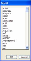
Step 4: The first sixteen of now
approximately 450 packages on the CRAN website.
As
mentioned in the lectures, the reason for not just pre-installing and then
loading all packages is that you would clog your computer’s memory with too
much stuff that you don’t need and hence suffer severe performance loss. If you
experiment with a number of packages and find that your computer becomes
somewhat sluggish, then you might want to unload packages. You do this with the
command
> detach(package)
You can
get rid off all packages except for the base package, which is essential for
running the RGui in the first place.
Step 5 Managing data
In the
course of an ![]() session, you will create a number of data
objects. That number is only limited by the size of your computer’s memory, but
as we have seen in the previous step, you may hit this boundary sooner than
expected. Under the Misc menu, you can list all
objects currently occupying your memory, and if you wish get rid of them. It
also lists the keyboard shortcut that helps you to cancel a computing intensive
operation, the <ESC> key.
session, you will create a number of data
objects. That number is only limited by the size of your computer’s memory, but
as we have seen in the previous step, you may hit this boundary sooner than
expected. Under the Misc menu, you can list all
objects currently occupying your memory, and if you wish get rid of them. It
also lists the keyboard shortcut that helps you to cancel a computing intensive
operation, the <ESC> key.
The Edit
menu is very much like what you know from other Windows programs. It also lists
the option to clear your console window.
![]() I strongly recommend that you don’t do that
because your console preserves the history of your complete R session. You will
use your console output as proof for your lab work. It also helps Jing Li understand what went wrong when you get stuck
during the lab exercises and you ask him for help.
I strongly recommend that you don’t do that
because your console preserves the history of your complete R session. You will
use your console output as proof for your lab work. It also helps Jing Li understand what went wrong when you get stuck
during the lab exercises and you ask him for help.
We have
talked a lot about memory during the last few steps. Program code (the
packages), data (objects) and the session history are all stored in memory and
together make up what is called your current workspace. You can dump (save)
your complete workspace to disk, thereby allowing you to continue a session
when you return some other time. That’s what is behind the Save Workspace and
Load Workspace options in the File menu. Similarly, you can save and load the
history of commands that you issue in a session. By the way, this history is
also accessible through the arrow up á key, which is particularly helpful
with long commands (having many parameters), where you made some small mistake.
Using the á key, you can recall a previous
command and edit the command.
Also under
the File menu, you set the current working directory, which by default is the
installation directory (which you are not allowed to write you in our Geography
labs). As a matter of fact, that’s something that you should make a habit.
Please either use the RGui File menu to change to a
directory on your U:\ drive or do the equivalent by typing on the console
> setwd(“U:/GTECH201/R”)
replace the string with a valid path to the folder of your choice)
Observe
that ![]() requires the path to be in quotation marks
(every
requires the path to be in quotation marks
(every ![]() object is either a
variable name, a number, or a text string, the latter is marked by the
enclosing quotation marks) and that the directories are separated by Unix-like forward
slashes even in a Windows environment.
object is either a
variable name, a number, or a text string, the latter is marked by the
enclosing quotation marks) and that the directories are separated by Unix-like forward
slashes even in a Windows environment.
Finally,
the Save to File… item of the File menu is what you
will use for your lab submission. With this, you save the contents of the
console window to a text file, which you will copy to your public_html
directory and set a link to, as part of your lab submission.
But now
let’s get started with ![]() proper.
proper.
Step 6
As
mentioned in the lecture, data input is not really a strong point of ![]() .
There is a variety of functions for reading external data but they all amount
to the use of data in ASCII format rather than convenient reading of native MS
Excel or dBASE formats, not to mention GIS data or
census data in SAS or SSS format.
.
There is a variety of functions for reading external data but they all amount
to the use of data in ASCII format rather than convenient reading of native MS
Excel or dBASE formats, not to mention GIS data or
census data in SAS or SSS format.
Download
and uncompress to a new directory on your U: drive the data
for this lab. Once you unzipped that file, you should among others have a
file ACTpop.txt in your R working directory. This file contains the population
figures n thousands for the
> ACTpop = read.table(“ACTpop.txt”,
header=TRUE)
This reads
in the data, and stores them in the data frame ACTpop.
Note the use of header=TRUE to ensure that ![]() uses the first line to get header information
for the columns. Type ACTpop at the command prompt,
uses the first line to get header information
for the columns. Type ACTpop at the command prompt,
> ACTpop
and the
contents of newly created ![]() object is printed in the console window.
object is printed in the console window.
Case is
significant for names of ![]() objects or commands. Thus ACTPOP is different
from ACTpop.
objects or commands. Thus ACTPOP is different
from ACTpop.
You can
now plot the ACT population between 1917 and 1997 by typing
> plot(ACT ~ Year, data=ACTpop, type=’p’, col=”black”, lwd=5)

Step 6: ACT population, in
thousands, at various times between 1917 and 1997.
ACT ~ Year is a graphics formula.
Read “Plot ACT (on the y-axis) against Year (on the x-axis).” The remaining
options determine plot type (here points), color, and size.
![]() Right-click inside the
graphics window. Observe that you can save the graphics to disk, or
alternatively copy it as a Windows metafile to the clipboard (the place
reserved in MS Windows memory for your copy and paste operations. You will need
to do this for your lab submission.
Right-click inside the
graphics window. Observe that you can save the graphics to disk, or
alternatively copy it as a Windows metafile to the clipboard (the place
reserved in MS Windows memory for your copy and paste operations. You will need
to do this for your lab submission.
We can use
data.frame()
to input data directly at the command line. The following assigns measurements
from an experiment, where by each amount by which an elastic band is stretched
over the end of a ruler, the distance that the band traveled upon release has
been recorded.
> elasticband = data.frame(stretch=c(46,54,48,50,44,42,52),
distance=c(148,182,173,166,109,141,166))
The
constructs c(46,54,48,50,44,42,52) and
c(148,182,173,166,109,141,166) concatenate or join the separate numbers into a
single vector object.
Step 7 Working with in-built data
An
important category of ![]() object is the data frame.
object is the data frame. ![]() uses data frames to
store rectangular arrays in which the columns may be vectors of numbers or
factors of text strings. Data frames are central to the way that
uses data frames to
store rectangular arrays in which the columns may be vectors of numbers or
factors of text strings. Data frames are central to the way that ![]() routines process data. Consider, for example,
the data frame cars
that is part of
the base package. It has two columns with the names speed and dist.
Typing summary(cars) gives summary information on these variables.
routines process data. Consider, for example,
the data frame cars
that is part of
the base package. It has two columns with the names speed and dist.
Typing summary(cars) gives summary information on these variables.
> data(cars) # Gives access to the
data frame cars
> summary(cars)
The #
character is used to write comments; anything after a # sign is not interpreted
by ![]() .
.
Step 8 Non-statistical data handling
There are
three common ways to extract subsets of vectors.
1. Specify the indices of the elements
that are to be extracted, e.g.
> x = c(3,11,8,15,12) # assign
five values to vector x
> x[c(2,4)] #extract elements in
positions 2 and 4 only
2. Use negative subscripts to omit the
elements
> x[-c(2,3)] # remove the
elements in position 2 and 3
3. Specify a vector of logical values.
The elements that are extracted are those for which the logical value is TRUE.
> x > 10
[1] FALSE TRUE
FALSE TRUE TRUE
> x[x > 10]
[1] 11 15 12
Another
way of accessing subsets is to look at data frames from a column or variable
perspective. The names() function can be used to
determine variable names. As an example, consider the
> data(airquality)
> names(airquality)
[1] “Ozone” “Solar.R” “Wind”
“Temp” “Month” “Day”
The sapply()
function is a useful tool for calculating statistics for each column of a data
frame. The first argument to sapply() is a data frame. The second is the name of a function
that is to be applied to each column. Consider the women data frame that also
is part of the base package:
> data(women)
> women # display the data
> sapply(women,mean)
![]() borrows many concepts
from Unix scripting languages. One is to abbreviate repetitive procedures by
identifying a pattern and then instruct
borrows many concepts
from Unix scripting languages. One is to abbreviate repetitive procedures by
identifying a pattern and then instruct ![]() to repeat the pattern n times. The colon : for instance, is used to mark the first and last element
of a list (similar to marking ranges in MS Excel).
to repeat the pattern n times. The colon : for instance, is used to mark the first and last element
of a list (similar to marking ranges in MS Excel).
> 5:15
[1] 5 6
7 8 9 10 11
12 13 14 15
This, by
the way, works also the other way around: 15:5 will generate the sequence in
reverse order. The colon : is a special form of a more
general function seq().
> seq(from=5, to=22, by=3) # the first value is 5, the last value is
<= 22
[1] 5 8
11 14 17 20
And to
repeat the sequence (2,3,5) four times over, enter
> rep(c(2,3,5), 4)
[1] 2 3
5 2 3 5 2
3 5 2
3 5
With this,
we came to the end of the introduction to ![]() .
The eight steps above provide you with all the information you need to now
perform the following six tasks, which make up your lab submission. Start Frontpage Express to create a new web page.
.
The eight steps above provide you with all the information you need to now
perform the following six tasks, which make up your lab submission. Start Frontpage Express to create a new web page.
![]() 1 Use
the data frame elasticband from step 6 to plot distance
against stretch. Copy the
graphics and paste it into your web page in Frontpage
Express.
1 Use
the data frame elasticband from step 6 to plot distance
against stretch. Copy the
graphics and paste it into your web page in Frontpage
Express.
![]() 2 The
aranda.txt dataset gives the size of the floor area (in ha) and the price (in
$000) for 15 houses in a local suburb in 1999.
2 The
aranda.txt dataset gives the size of the floor area (in ha) and the price (in
$000) for 15 houses in a local suburb in 1999.
(a) Plot sale.price versus area
(b) Use the histogram parameter to plot a histogram of the sale prices.
Copy both graphs to your web page.
![]() 3 The
orings.txt data frame gives data on the damage that had occurred in
3 The
orings.txt data frame gives data on the damage that had occurred in
Create a new data frame by extracting these rows from orings.txt and plot Total incidents against Temperature for this new data frame.
Obtain a similar plot for the full dataset. Copy both graphs to your web page.
![]() 4 Import
the lakes.txt dataset containing the elevation of lakes in
4 Import
the lakes.txt dataset containing the elevation of lakes in
Assign the names of the lakes using the row.names
function. The following is a list of the lake names:
Then obtain a plot of lake area against elevation and copy the graph to your
web page.
![]() 5 Using
the sum() function, obtain a lower bound for the area
of
5 Using
the sum() function, obtain a lower bound for the area
of
![]() 6 The ^
symbol denotes exponentiation. Consider the following:
6 The ^
symbol denotes exponentiation. Consider the following:
>
1000*((1+0.075)^5 – 1) # interest on
$1,000, compounded annually
# at 7.5% per annum for five years
(a) Type the above expression
(b) Modify the expression to determine the amount of interest paid of the rate
is 3.5%
(c) What happened is the exponent 5 is replaced by seq(1,
10)?
Record your observation in your web page.
Rename
your web page lab08.answers.html and set a link to this page from your home page.
Then send an email to Jing Li announcing your lab
submission and providing him with the URL to your lab answers.