Lab 6
Transforming
Spatial Data
Objectives:
By the end of this lab you
will be able to:
·
Digitize
vectors on an image backdrop
·
Compare rasters and vectors
·
Create
metadata
·
Georeferencing an
image
Preparatory step: Open a
text editor such as Notepad and save the empty document to you U:\ drive,
giving it the name [your login name]_lab6.txt.
Whenever you find something marked in red in the
reminder of these lab instructions, type your answer into you text document and
save it to disk. At the end of the lab, you will be asked to attach the text
document to an email to Jing
Li.
1.
Digitizing
vectors on an image backdrop
This task consists of two
parts. First you will be digitizing parts
of the shoreline of the
Before you continue
with this lab, please create a new folder called Lab6Data on C:\temp or in your
own U:\ directory, and copy all of the files from the scratch drive (S:\GTECH201\Labs\Lab6Data)
into this new folder.
a)
Start both ArcCatalog and ArcMap
b)
Within
ArcCatalog, connect to the Lab6Data folder you just created using the
"Connect to Folder" button at the top of the window (looks like a
globe with an arrow in front of it)
c)
Click on the
raster file (downtown_dc.bil) and drag it into
the legend pane of ArcMap. This image is a satellite image of downtown
This file has not yet been geo-referenced (you will do that later). For now
just ignore the warning and click <OK>.
d)
Within ArcCatalog, create new shapefile
by clicking on: File-New-Shape file
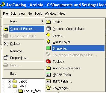
·
name it potomac
·
let it be of
type polyline
·
and click
<ok>
·
Drag the potomac shapefile
from ArcCatalog into the Legend pane of ArcMap. Make
sure that potomac.shp is the top-most layer. If
it isn't, drag it and drop it until it is the top layer in the table of
contents.
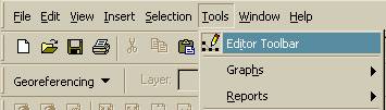
e)
In ArcMap open the EditorToolbar
if it is not already open
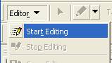
Then start an edit session to edit the new shapefile
f)
Click on the
arrow next to the button with the Pencil on the EditorToolbar
and click on Create New Feature (the Pencil Icon)
·
start drawing
your line by single clicking along the eastern edge of the Potomac river near
when the I-66 bridge (the northern-most bridge over the
·
trace the river's edge by single clicking along the
shoreline. You may want to experiment with zooming in and out to find the image
resolution that works best to follow the river’s edge.
·
after a couple
of points, right-click anywhere on the screen to see your range of options
·
observe the difference between right-clicking away from
the line you are drawing (your digitized feature) and right-clicking on a point
you made (a vertex).
·
you can also
use the pan tool while you are digitizing by clicking on the pan button (looks
like a hand) moving around the image and then continue by clicking the pencil
button again and clicking to make more points along the river
·
move your way down the river's edge until you get to
the
·
when you are finished right-click on the last vertex
and click Finish-Sketch.
g)
Click Editor –
Save Edits
h)
Now locate the
bend of the
·
Now move the
cursor (but be careful) to follow the new stretch of coastline.
·
Once you are
finished, double-click.
·
As you can
see, the fast drive lives dangerously.
i)
Click Editor -
Stop Editing. Remember to click on "Yes" when the program asks you if
you want to save your changes.
The second part of this
task is to construct new features. For this, your need
to zoom into the area immediately surrounding the
Don’t spend more than 10
minutes on this task. Make sure that you stop editing and save your results!
2.
Saving
a map
You have made
a lot of changes to this map. Because you want to keep the new map that you have
created and also keep the old template map, you will use Save As to save this
map under a new name.
a)
Click
File and click Save As.
b)
Navigate to
the Lab6Data directory.
c)
Type CapitolHill (no spaces!). Click Save.
3.
Raster
– vector comparison
Not a true comparison at
this stage. You will do this at the end of the lab. However, in this task you
are supposed become familiar with issues of data quality and the difficulty of
getting a handle on it. Again, we have two parts. First,
![]() Count the number of houses just to the east
of Union Station and write
Count the number of houses just to the east
of Union Station and write
your answer into your text document.
At this step you are asked to provide
three answers (a, b, c).
This sounds like an easy
task. But try it for yourself. To make it less challenging, (a) just count the houses on the first square block
due east of Union Station. Hint: play with the zoom level; sometimes being too
close makes it harder. When you write your answer in a text file that you will
submit, include a few words of comment as to what made you choose one shadow as
a house and others as garages or trees.
Now zoom in around
the
4.
Creating
metadata
Let’s familiarize
ourselves again with the concept of metadata. Switch to ArcCatalog,
select any of the Lab6 geography files in the Lab6Data folder in your class
workspace and look at their metadata tabs.
![]() What categories of metadata are there? Note
your answer in your text document.
What categories of metadata are there? Note
your answer in your text document.
![]() Click on the spatial metadata tab and tell us
(in your text file) everything you can learn about the coordinate system used
for
Click on the spatial metadata tab and tell us
(in your text file) everything you can learn about the coordinate system used
for
i) the Roads
file (MSARds.shp)
ii) the Fire Department file (dcfrdgeo.shp)
iii) the aerial, Potomac, or DCBuildings files
a)
In ArcCatalog, select the DC Fire Department file (dcfrdgeo.shp) and look at its metadata.
b)
c)
Click the
Fields tab and select the second row called Shape. It tells you that the projection
is undefined. The lower window of that Fields tab has a field property called
Spatial Reference with an ellipsis ![]() to its right. Click
the ellipsis and then click on "Select..." (select
a predefined coordinate system).
to its right. Click
the ellipsis and then click on "Select..." (select
a predefined coordinate system).
i.
select it from
the Projected Coordinate Systems
ii.
double-click
the UTM folder, then double-click the NAD 1983 folder, and finally select
"NAD 1983 UTM Zone 18N.prj" and click Add
iii.
all its
parameters have already been defined by ESRI
d)
Click OK to
close the Spatial Reference Properties box, then OK to close the Shapefile Properties dialog box
e)
You can verify
the new coordinate system in the metadata. Click View - Refresh, then click the Spatial tab.
5.
Geoeference the aerial image
At this stage, the image
is just that, dumb data without any reference to the real world, nothing that
we could use in a
The basic procedure is to
move the image into the same space as the target data by identifying a series
of ground control points of known x, y coordinates. A combination
of one control point on the image and the corresponding control point on the
target data is called a link. If possible, you should spread the links out over
the entire image.
The degree to which the
transformation can accurately map all control points can be measured by
comparing the actual location of the map coordinate to the transformed position
in the raster. The distance between these two points, known as residual error,
is computed by taking the root mean square sum (RMS) of all the residuals.
a)
Start with a
complete new project in ArcMap (the safest way to assure this is to exit ArcMap
and to restart it again).
b)
Load the
c)
In the table
of content, right-click MSARds and click Zoom to
Layer
d)
Add the aerial
image to your project.
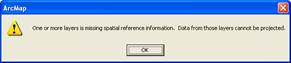
Click OK when the window opens and lets you know your files are missing spatial
reference information. Right-click downtown_dc.bil
in the table of contents and click Zoom to Layer.
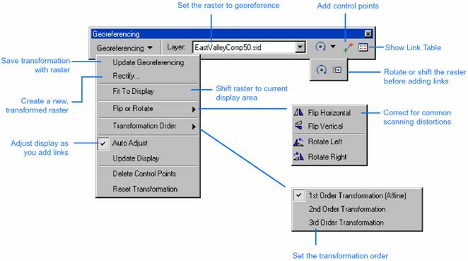
e)
Right-click
the View menu, point to Toolbars, and click Georeferencing.
From the Georeferencing toolbar, click the Layer
dropdown arrow and click the image layer you want to georefence
(you should have only one option, downtown_dc).
f)
Click Georeferencing and then click Fit To
Display.
This will display the image in the same area as the target layers. You can also
use the Shift and Rotate tools to move the image as needed.
g)
Click the Control
Points tool to add control points.
h)
To add a link,
click the mouse over a known location on the image, then over a known location
on the MSARds layer. You may find it useful to use a
Magnification window to add your links in. Choose easily recognizable points
like road intersections or sharp edges to link points on the image with their
corresponding points in the roads layer. Press the Esc key to remove a link
while you are in the middle of creating it.
i)
Add ten links
j)
Click View
Link Table to evaluate the transformation. You can examine the residual error
for each link and the RMS. If you are satisfied with the registration, you can
stop entering links. You can delete an unwanted link from the Link Table dialog
box.
k)
Click Georeferencing and click Update Georeferencing
to save the transformation information with the image. This creates a new file
with the same name as the image but with an .aux extension.
Now you are ready to print
a copy of this map.
6.
Printing
your map
You can easily print the maps you have
composed in ArcMap, however for lab submission you are not
required to print your map. The Layout view lets you arrange map elements, such as data
frames, scale bars, and North arrows, on the page exactly as you want them to
print.
a)
Click
File and click Print.
b)
Click OK.
7.
Export
map and wind down
a)
To Export your
map, click File/Export Map and then make sure you select pdf
as the file type
b)
Click File and
click Exit, or simply click the Close button (x) in the upper-right corner of
the ArcMap window. Do the same for ArcCatalog.
This concludes Lab 6. Submit your answers recorded in a text file
and the pdf as an email attachment to Jing
Li.